Probability is the extension of logic from \(\set{0,1}\) to \([0,1]\); it lets us quantify uncertainty.
The Basics
An outcome is a single possibility of an experiment, e.g. rolling a 6 on a die. The sample space\(S\) is the set of possible outcomes. An event\(A\) is a subset of the sample space, presumably with an interpretable meaning, e.g. rolling an even number on a die.
So, \(\mathcal{P}(S)\) is the set of possible events. This includes \(\varnothing\) and \(S\) itself.
\(S\) may be discrete (e.g. \(\mathbb{N}\)) or continuous (e.g. \(\mathbb{R}\))
Since events are sets, they can be constructed with set-theoretic notation and operations: complement, union, intersection. Mutually exclusive events correspond to disjoint sets.
Discrete Probability Model
A probability model defines all the possible sample points and defines how probabilities are assigned to them. It defines a probability function\(P:\mathcal{P}(S)\to [0,1]\) that maps events to their probabilities.
Axioms of Probability (first-principles version)
Definition
Probabilities are between \(0\) and \(1\): \(0\geq P(A)\geq 1\)
Probability of an outcome occurring is \(1\): \(P(S)=1\)
Probability distributes over disjoint events: \(P\left(\displaystyle\bigcup_{i=1}^{\infty}A_i\right)=\displaystyle\sum\limits_{i=1}P(A_i)\)
The null event has probability \(0\): \(P(\emptyset)=0\).
A more formal model of probability is derived in [[Unit 2a - Formalizing Probability]]
The conditional probability\(P(A\mid B)\) of event \(A\) given \(B\) is the probability of \(A\) occurring if we know that \(B\) has occurred. We have, for \(P(B)\geq 0\), \[P(A\mid B)=\dfrac{P(A\cap B)}{P(B)}\]
Here, \(P(B)\) in the denominator normalizes the probability of \(A\cap B\) by the probability of \(B\) occurring at all. If \(P(A\cap B)\) is really small but \(P(B)\) is also small, \(P(A\mid B)\) shouldn't be that small.
Two events \(A\) and \(B\) are independent when knowing information about whether one has occurred doesn't give you information about whether the other has occurred. So, we would have \(P(A\mid B)=P(A)\).
Complements of Events
For event \(A\), the complement\(\bar{A}:=S\setminus A\) is the event that \(A\) does not occur. The complement rule\(P(\bar{A})=1-P(A)\) states that the probability of an event \(A\) occurring is the inverse (wrt. \(1\)) of the probability of \(A\) not occurring, i.e. the probability of the complement.
The complements of intersections and unions are described by De Morgan's laws:
Complement of intersection: \(P(\overline{A\cap B}) = P(\bar{A} \cup \bar{B})\)
Complement of union: \(P(\overline{A\cup B}) = P(\bar{A} \cap \bar{B})\)
Intersections of Events
The intersection of two events is the event that they both occur.
The probability of an intersection of two events \(A\) and \(B\) is \(P(A\cap B)=P(B\mid A)P(A)\), and so by symmetry \(P(A\cap B) = P(A\mid B)P(B)= P(B\mid A)P(A)\) (product rule). If \(A\) and \(B\) are independent, we have \(P(A\mid B)=P(A)\), so \(\boxed{P(A\cap B)=P(A) P(B)}\) for independent \(A,B\).
By extension, we have \(P\left(\displaystyle\bigcap_{i=1}^{k} A_i \right)=\displaystyle\prod_{i=1}^k P\left(A_i\mid \displaystyle\bigcap_{j=1}^{i-1}A_j\right)\). This can be derived by induction.
Unions of Events and Inclusion-Exclusion
The union of two events is the event that at least one of them occurs.
The probability of a union of two events \(A\) and \(B\) is \(P(A\cup B)=P(A)+P(B)-P(A\cap B)\). If \(A\) and \(B\) are mutually exclusive, we have \(P(A\cap B)=0\), so \(\boxed{P(A\cup B)=P(A)+P(B)}\) for mutually exclusive \(A,B\).
Note: mutual exclusivity is not independence. In fact, mutual exclusion implies strong dependence because knowing event \(A\) occurred tells you with complete certainty that event \(B\) did not occur
By extension, we have \(P\left(\displaystyle\bigcup_{i=1}^{k} A_i \right)=\displaystyle\sum\limits_{i=0}^k\left( (-1)^{i-1} \underset{\underset{|I|=i}{I\subseteq\set{1\dots k}}}{\sum} \displaystyle\bigcap_{j\in I} A_j \right)\), which is the probability form of the inclusion-exclusion principle. It can be derived and proved inductively/recursively.
In the \(k=3\) case, we have \(P(A\cup B\cup C)=P(A)+P(B)+P(C)-P(A\cap B)-P(A\cap C)-P(B\cap B)+P(A\cap B\cap C)\)
Partitioning the Sample Space
The law of total probability states that if events \(E_1\dots E_k\) partition the sample space then for any event \(A\), we have \(P(A)=\displaystyle\sum\limits_{i=1}^{k}P(A\cap E_i)=\sum\limits_{i=1}^{k}P(A\mid E_i)P(E_i)\).
Informally, the probability of an event \(A\) occurring gets "distributed" over all the possible partition cells. Every outcome in \(A\) must occur in exactly one of the partitions, so adding the probability of \(A\) in each partition yields its total probability.
Bayes' Theorem
From the law of total probability, \(P(A\mid B)P(B)=P(A\cap B)=P(B\cap A)=P(B\mid A)P(A)\), so \(P(A\mid B)P(B)=P(B\mid A)P(A)\) and thus \(\boxed{P(A\mid B)=\dfrac{P(B\mid A)P(A)}{P(B)}}\); this is Bayes' theorem. So, Bayes' theorem relates \(P(A\mid B)\) and \(P(B\mid A)\).
\(P(A\mid B)\) is the posterior; it is what we are solving for
\(P(B\mid A)\) is the likelihood
\(P(A)\) is the prior; it describes how likely \(A\) is to occur in general. This is general "background knowledge" that conditions the estimate
\(P(B)\) is the evidence; it normalizes the posterior. Often, we use the law of total probability to calculate it.
Bayes' theorem is useful for questions involving observations and conclusions. We often know the probability that evidence will have presented itself if an event has occurred, and we wish to determine the probability of the event having occurred given we have observed evidence. This lets use "invert" problems in a useful way.
In machine learning, we often wish to calculate \(P(\vec{w}\mid \mathcal{D})\), the probability that our estimate \(\vec{w}\) is correct given training data \(\mathcal{D}\); this lets us pick the estimate with the highest likelihood of being correct. Bayes' theorem lets us calculate this in terms of \(P(\mathcal{D}\mid \vec{w})\) (the probability of observing the data we did given our estimate), \(p(\vec{w})\) (a prior whose distribution we pick), and \(P(\mathcal{D})\) (an ignorable constant factor describing the "quality" of the data).
Unit 2a - Formalizing Probability
Unit 3 - Discrete Random Variables
The Basics
A (discrete) random variable is a function \(X : S\to \mathbb{R}\) mapping each outcome in \(S\) to a real number.
E.g. \(X\) is the square root of the face value rolled on a die (\(S=\set{1\dots 6}\))
E.g. \(X\) is the sum of three independent die rolls (\(S=\set{1\dots 6}\times \set{1\dots 6}\times \set{1\dots 6}\))
The probability mass function (PMF) of a discrete random variable \(X\) is the function \(p_X(x)\) defined by \(p_X(x):=P(X=x)\). Given input \(x\), the PMF returns the probability of the random variable having that value.
Thus, the axioms of probability apply to \(p_X\) by inheritance (check)
Generally, we drop the subscript and just refer to the probability mass function as \(p\)
The cumulative distribution function (CDF) \(F_X(x)\) of discrete random variable \(X\) is the function \(F_X:\mathbb{R}\to [0,1]\) defined by \(F_X(x):=P(X\leq x)\) for \(-\infty < x < \infty\). Given input \(x\), the CDF returns the probability that the random variable has value smaller or equal to \(x\).
We can compute \(P(X\in (a,b])\) for \(a\leq b\) by computing \(F_X(b)-F_X(a)\), à la fundamental theorem of calculus II.
Since probabilities are always positive, \(F_X\) is a totally non-decreasing function. So, \(x_1 < x_2\implies F_X(x_1)\geq F_X(x_2)\) for all \(x_1, x_2 \in \mathbb{R}\).
We have \(F_X(-\infty)=\lim\limits_{x\to -\infty}F(x)=0\) and \(F_X(\infty)=\lim\limits_{x\to \infty}F(x)=1\)
Common uses of random variables in probability questions:
Modelling costs of processes
Defining prizes for games
Note: what we are considering here are discrete random variables. Results and distributions will be generalized to include continuous random variables later.
Expectation
The expected value\(\mathbb{E}\left[X \right]\) of random variable \(X\) is the most error-minimizing prediction for its value; it is a general version of the mean. We have \(\mathbb{E}\left[f(X) \right]=\displaystyle\sum\limits_{s\in S}f(s)p_X(s)\). In "raw" case where \(f\) is the identity function, we have \(\mathbb{E}\left[X \right]=\displaystyle\sum\limits_{s\in S}s p_X(s)\).
The expected value has the following properties:
Constants are expected to be themselves: \(\mathbb{E}\left[c \right]=c\) for constant \(c\)
Behavior under affine transformation: \(\mathbb{E}\left[aX + b \right]=a \mathbb{E}\left[X \right]+b\)
Sums of random variables: \(\mathbb{E}\left[\displaystyle\sum\limits_{i=1}^{k} f_i(X_i) \right]=\displaystyle\sum\limits_{i=1}^{k} \mathbb{E}\left[f_i(X_i) \right]\)
The expected value gives us a good idea of the "centre" of the distribution of \(X\).
==independent product E[XY] = E[X]E[Y]
center of mass/centroid==
Variance
The variance\(V\left[X \right]\) of random variable \(X\) measures how far we expect a randomly sampled value to be from the mean. Literally, we have \(V\left[X \right]:=\mathbb{E}\left[(X - \mathbb{E}\left[X \right])^2 \right]\). A derivation from this that is useful for computation is \(\boxed{V\left[X \right]:=\mathbb{E}\left[X^{2} \right]-(\mathbb{E}\left[X \right])^{2}}\).
The standard deviation of \(X\) is the square root of its variance, i.e. \(\sigma_X := \sqrt{V\left[X \right]}\).
Variance has the following properties:
Constants don't vary: \(V\left[c \right]=0\) for constant \(c\)
Behavior under affine transformation: \(V\left[aX+b \right]=a^{2}V\left[X \right]\).
Non-negativity: \(V[X]\geq 0\) for all random variables \(X\). If you get negative variance, you have fucked up!
If random variables \(X_1, \dots, X_k\) are independent, then the variance of their sum is the sum of their variances, i.e. \(V\left[\displaystyle\sum\limits_{i=1}^{k} f_i(X_i) \right]=\displaystyle\sum\limits_{i=1}^{k} V\left[f_i(X_i) \right]\).
==The variance gives us a good idea of the "spread" of the distribution of \(X\).==
Discrete Distributions
Some "types" of discrete random variables are frequent and useful enough that we hard-code them into our understanding of probability. This way, we can describe useful quantities like expected value, variance, etc. in general, i.e. in terms of the parameters.
The Bernoulli Distribution
The Bernoulli distribution\(\text{Bernoulli}(p)\) models a Bernoulli trial: an experiment where success occurs with probability \(p\), and thus failure occurs with probability \(1-p\). A random variable \(X\sim \text{Bernoulli}(p)\) will be \(1\) with probability \(p\) and \(0\) with probability \(1-p\).
Probability mass function: \(p(x)=p^{x}(1-p)^{1-x}\) for \(x\in \set{0,1}\)
Expected value: \(\mathbb{E}\left[X \right]=p\)
Variance: \(V\left[X \right]=p(1-p)\)
There really isn't more to say because this distribution is piss simple.
The Binomial Distribution
The Binomial distribution\(\text{Binomial}(n,p)\) models the number of successes seen in \(n\) successive independent Bernoulli trials with probability \(p\).
Probability mass function: \(p(x)=\displaystyle{n\choose x}p^{x}(1-p)^{n-x}\) for \(x\in \set{0, 1, \dots, n}\)
Expected value: \(\mathbb{E}\left[X \right]=np\)
Variance: \(V\left[X \right]=np(1-p)\)
derivation
Note: the Bernoulli distribution is the special case of the binomial distribution where \(n=1\).
The sum of binomial random variables is also a binomial random variable if the probabilities are all the same. So, for \(\displaystyle Y\sim\sum\limits_{i=1}^{k}Y_i\) where random variables \(Y_i\sim \text{Binomial}(n_i, p)\), we have \(Y\sim \text{Binomial}\left(\displaystyle\sum\limits_{i=0}^{k}n_i, p\right)\).
In the \(n=1\) case, we have that the sum of \(n\) Bernoulli trial RVs with probability \(p\) is an RV with distribution \(\text{Binomial}(n,p)\).
The Geometric Distribution
The geometric distribution\(\text{Geometric}(p)\) models the number of Bernoulli trials with probability \(p\) that occur until a success is observed. Note: the input counts the failures and the final success, not the just failures.
Probability mass function: \(p(x)=(1-p)^{x-1}p\) for \(x\in \mathbb{N}\).
Cumulative distribution function (i.e. \(P(X \geq x)\)): \(F(x)=1-(1-p)^{x}\)
If we observe the first success (which has probability \(p\)) on the \(x\)th trial, there must have been \(x-1\) failures (which each have probability \(p-1\)) right before it. So, by the product rule, the probability of all of this happening in conjunction is \((1-p)^{x-1}p\).
There isn't a bound on how many failures can occur; although improbable, an arbitrary number of failures can happen in a row. So, the geometric distribution is defined for all \(\mathbb{N}\) in the same way as a geometric series, which is where it gets its name.
The geometric distribution is memoryless; the probability of a success doesn't depend in any way on how many failures occurred before. Formally, \(P(X > a+b\mid X > a)=P(X > b)\).
The expected time until the first success in a binomial distribution \(\text{Binomial}(n, p)\) follows the geometric distribution \(\text{Geometric}(p)\).
The Negative Binomial Distribution
The negative binomial\(\text{Negative-Binomial}(r, p)\) models the number of Bernoulli trials with probability \(p\) that occur until the \(r\)th success is observed.
Probability mass function: \(p(x)=\displaystyle{{x-1}\choose r-1}p^{r}(1-p)^{x-r}\) for \(y=r+\mathbb{N}\)
Note: The geometric distribution is a special case of the negative binomial distribution where \(r=1\).
The \(p^{r}(1-p)^{x-r}\) sub-expression is the probability of exactly \(r\) successes and \(x-r\) failures; the \(\displaystyle{{x-1}\choose r-1}\) corresponds to the number of ways to select where the \(r-1\) failures occur in the sequence of \(x-1\) trials. Note that we use \(r-1\) and \(x-1\) instead of \(r\) and \(x\) because we know the final success must be the last trial in the sequence.
The Poisson Distribution
The Poisson distribution \(\text{Poisson}(\lambda)\) models the number of events that occur in a fixed time period where there is an average of \(\lambda\) events per period and probability of an event does not depend on the time since the last event. Here, we assume time is continuous. So, \(X\sim\text{Poisson}(\lambda)\) if \(X\) models the number of such events that occurred in the time period.
Probability mass function: \(p(x)=\dfrac{\lambda^{x}}{x!}e^{-x}\) for \(x\in \mathbb{N}\) and \(\lambda > 0\)
The sum of independent Poisson random variables is also a Poisson random variable. Specifically, for \(\displaystyle Y=\sum\limits_{i=1}^{k}Y_i\) where random variables \(Y_i\sim \text{Poisson}(\lambda)\), we have \(Y\sim \text{Poisson}\left(\displaystyle\sum\limits_{i=0}^{k}\lambda_i\right)\).
The Poisson distribution can be approximated by a binomial distribution with large \(n\) and small \(p\). Specifically, \(\text{Poisson}(np)\approx \text{Binomial}(n,p)\).
Informal explanation: successes can occur anywhere in the sequence of Bernoulli trials implied by the binomial distribution. When \(n\) is large and \(p\) is small, the discretization error becomes small enough to model uniformity over a continuous range.
This is useful for computer modelling because computing combinatorial probability can involve prohibitively large and expensive integers. Approximating with a poisson distribution solves this problem
put stat 230 stuff here
For Poisson RV \(X\sim \text{Poisson}(\lambda)\), we may wish to consider the RV \(X_t\) counting the number of successes over some sub-period of time-length \(t\). If successes are independent, never occur at the same time, and happen at a constant rate, then \(X_t\) also follows a Poisson distribution given by \(X_t\sim \text{Poisson}(\lambda t)\).
So, under these assumptions, we can partition a time period into multiple sub-periods and model event counts in these periods as Poisson distributions proportional to \(X\)
The Hypergeometric Distribution
The hypergeometric distribution\(\text{Hypergeometric}(N, r, n)\) models the number of successes in a random sample without replacement of \(n\) elements from \(N\) elements where \(r\) are successes.
Probability mass function: \(p(x)=\displaystyle\left.{r\choose x}{N-r\choose n-x} \middle/ {N\choose n}\right.\)
Variance: \(V\left[X \right]=\displaystyle n \left(\dfrac{r}{N}\right)\left(\dfrac{N-r}{N}\right)\left(\dfrac{N-n}{N-1}\right)\)
For very large \(N\), \(r\) and modest \(n\), \(\text{Hypergeometric}(N, r, n)\approx \text{Binomial}\displaystyle\left(n, \frac{r}{N}\right)\). The idea is that, as \(N\) and \(r\) become large, the effect of not replacing draws becomes negligible. Thus, successive draws can be reasonably modelled as independent Bernoulli trials with probability \(r/N\).
maybe reformat the data stuff as a table (e.g. the CDF, etc). use llm to quickly reformat.
Motivation
A continuous random variable\(Y\) is a random variable \(Y:S\to \mathbb{R}\) such that its CDF \(F_Y: \mathbb{R}\to [0,1]\) is a continuous function. Continuous random variables define distributions that are not discrete, so \(S\) cannot be a discrete set.
Non-discrete sample spaces immediately raise a problem: if we single points \(s\in S\) have non-zero probabilities (i.e. \(P(s)\geq 0\)), then \(\displaystyle\sum\limits_{s\in S}p_Y(s)\) will be infinite (and thus larger than \(1\)), violating the axioms of probability. But, if each \(s\in S\) does indeed have probability \(0\), the probability mass function will be zero everywhere and therefore useless for encoding the distribution.
Somehow, we seem to need to add up infinitely many \(0\)s to get something that's not a \(0\). This suggests some calculus trickery is involved
Probability Density Functions
To solve this issue, we introduce the concept of a probability density function\(p_Y(y)\), which is the derivative of the CDF: \(p_Y(y):=\dfrac{\text{d}}{\text{d}y}F_Y(y)\). Instead of evaluating it directly, we retrieve probabilities by integrating over it: \(P(a\leq Y\leq b)=\displaystyle\int_{a}^{b}p_Y(y)\,\text{d}y=F_Y(b)-F_Y(a)\).
Note that the PDF is not zero everywhere like the corresponding PMF would be: the value of the PDF at point \(y\) can be interpreted as the probability of landing in a small region \((y-\text{d}y, y+\text{d}y)\) normalized by its size, i.e. \(\lim\limits_{\varepsilon\to 0}\dfrac{P(y-\varepsilon \leq Y \leq y+\varepsilon)}{\varepsilon}\). Thus, it encodes the relative pull of probability towards \(y\); the name "probability density function" is apt.
Properties
Some other properties of probability density functions include:
Positivity: \(p_Y(y)\geq 0\) for \(-\infty < y < \infty\)
Total probability: \(\displaystyle\int_{-\infty}^{\infty}p_Y(y)\, \text{d}y=1\)
Outcomes are probability \(0\): \(P(Y=a)=\displaystyle\int_{a}^{a}p_Y(y)\,\text{d}y=0\)
Armed with probability density functions, we will see that extending probability to continuous structures is a matter of swapping out discrete concepts for continuous ones, e.g. swapping sums for integrals.
Expected Value and Variance
The expected value of continuous random variable \(Y\) is \(\mathbb{E}\left[Y \right]=\displaystyle\int_{\infty}^{\infty}y\,p_Y(y)\,\text{d}y\). This generalizes to \(\mathbb{E}\left[g(Y)\right]=\displaystyle\int_{\infty}^{\infty}g(y)\,p_Y(y)\,\text{d}y\) for \(g : \mathbb{R}\to \mathbb{R}\). Its variance is formally defined as \(\mathbb{E}\left[(Y-\mathbb{E}\left[Y \right])^{2} \right]=\displaystyle\int_{-\infty}^\infty(y-\mathbb{E}\left[Y \right])^{2} p_Y(y)\,\text{d}y\); variance identities like \(V\left[Y \right]=\mathbb{E}\left[Y^2 \right]-(\mathbb{E}\left[Y \right])^2\) still hold.
Percentiles and the Median
The \(p\)th quantile (or \(100p\)th percentile) \(\pi_p\) of continuous random variable \(Y\) is the value \(\pi_p\) such that \(F_Y(\pi_p)=p\), where \(0 < p < 1\). The \(50\)th percentile is called the median, denoted \(\text{Median}[Y]\).
So, for continuous distributions, \(\text{Median}[Y]\) is the value such that \(P(Y\geq \text{Median}[Y])= \dfrac{1}{2}\)
We define the interquartile range (IQR) as \(\pi_{0.75}-\pi_{0.25}\).
So, to solve directly for the \(p\)th percentile, we evaluate the equation \(\displaystyle\displaystyle\int_{-\infty}^{a} f(y) \, \text{d}y=p\).
Moment Generating Functions
The moment generating function (MGF) \(m_Y : \mathbb{R} \to (\mathbb{R}\to \mathbb{R})\) of random variable \(Y\) is defined as \[m_Y(t)=\mathbb{E}\left[e^{tY} \right]=\begin{cases}\displaystyle\sum\limits_{y\in Y}e^{tY}p_Y(y) &\text{for discrete $Y$} \\ \displaystyle\int_{-\infty}^{\infty}e^{tY}p_Y(y) \, \text{d}y &\text{for continuous $Y$}\end{cases}\]
. If \(m_Y\) exists, it is unique; \(m_X=m_Y\) implies that \(F_X=F_Y\), and further that \(X\) and \(Y\) are different spellings of the same random variable (isomorphic?).
??
part of this is the whole addition becomes multiplication homomorhpism introduced by making everything exponential; perhaps this is why everything is exponential
in this section
what are momenets, central moments
expected value as first moment, variance as second central movement
general motivation for moments and mgfs
primer on generating functions
mgf definitions
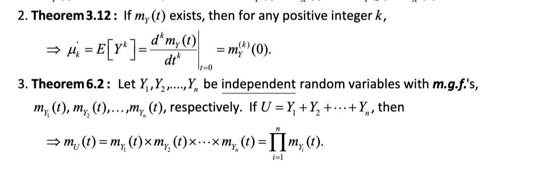
theorems from the screenshot and beyond (figure out the weird notation in the screenshot)
motivation: the idea is basically that moment generating functions are a "canonical form" of distributions; they completely describe the distribution in an algebraic way, similar to the probability density function. But, the mechanics of working with these functions is easier than working with MGFs in a few ways: FIGURE OUT. So, they are more pragmatic as objects representing distributions that can be manipulated with the rules of algebra. One reason might be that they encode moments directly, e.g. the mean directly, so they are more easily integrated with the point estimates like expected value and variance that we work with commonly.
we will see results about sums and linear combinatoins of random variables. these can be derived by writing the MGFs of the distributions, summing (or whatever) the expressions, then re-interpreting / re-casting / pattern-matching the result to another MGF. why is this easier with MGFs than PFs? probably has to do with sum of RVs becomes product of MGFs due to the e to the x thing I think. suss out properly.
MGFs are exponential generating functions I think.
==use these as a question answering trick for solving expectations with \(e^X\) type stuff. Remember log and exponent rules to manipulate the equations and stuff. this includes change of base for logs so you could calculate \(E[b^X]\) for base \(b\).
Continuous Distributions
Again, some types continuous random variables come up enough to cache them as distributions.
We will see that many continuous distributions are analogous to some discrete distribution; think of them as a limit \(n\to \infty\) case of the discrete distribution.
We also note that all continuous distribution PMFs are defined over \((-\infty, \infty)=\mathbb{R}\). Often, the PMFs are only nonzero over a sub-interval of \(\mathbb{R}\). To avoid typesetting piecewise functions everywhere, we adopt the notational convention that PMFs are \(0\) wherever they are not explicitly defined.
The Uniform Distribution
The Uniform distribution\(\text{Uniform}(a, b)\) models a random variable that has an equal likelihood of being any value between \(a\) and \(b\) where \(a < b\).
Probability density function: \(p_Y(y)=\dfrac{1}{b - a}\) for \(a < y < b\).
Cumulative distribution function: \(F_Y(y)=\dfrac{y-a}{b - a}\) for \(a < y < b\), \(0\) for \(y < a\), \(1\) for \(y > b\).
Uniform distributions behave nicely under affine transformation: \(a \text{Uniform}(a, b)+b\sim \text{Uniform}(aa + b, a b + b)\). We can derive results like this by plugging the expression into the CDF or MGF (since both uniquely define the distribution) and using algebraic manipulation to transform them into something that matches the CDF or MGF of a single distribution.
Note: The sum of two uniform distributions is not a uniform distribution, but an Irwin-Hall distribution.
There is also a discrete uniform distribution, where a point is sampled from a range partitioned into discrete buckets.
The Normal Distribution
The big cheese
The normal distribution or Gaussian distribution\(Y\sim \text{Normal}(\mu, \sigma^{2})\) models, well, a lot of things.
Probability density function: \(p_Y(y)=\dfrac{1}{\sigma\sqrt{2\pi}}\exp{\left(-\dfrac{1}{2 \sigma^{2}}(y-\mu)^{2}\right)}\)
Moment-generating function: \(m_Y(t)=\exp{\left(\mu t + \dfrac{1}{2}\sigma^{2}t^{2}\right)}\)
Expected value: \(\mathbb{E}\left[Y \right]=\mu\)
Variance: \(V\left[Y \right]=\sigma^{2}\)
Note that we don't have a nice cumulative distribution function other than the integral definition \(\Phi\). This is because the indefinite gaussian integral\(\displaystyle \displaystyle\int\exp{(x^2)} \, \text{d}x\) is not solvable (although the definite integral \(\displaystyle \displaystyle\int_{-\infty}^{\infty}\exp{(x^2)} \, \text{d}x\) is famously equal to \(\sqrt{\pi}\)). In practice, we can calculate increments of this integral numerically and retrieve them from a Z-table.
But why is pi here? 3b1b video
Z-tables and the Standard Distribution
We define the standard normal random variable\(Z\) as a normal random variable with mean \(0\) and variance \(1\), i.e. \(Z\sim \text{Normal}(0, 1)\). A z-table is a list of numerical values for the CDF of \(Z\) some range starting at \(0\); the most detail is given around \(0\).
We use Z-tables to compute probabilities involving normal distributions by re-mapping our particular instance of the normal distribution onto the standard one. Specifically, for \(Y\sim \text{Normal}(\mu, \sigma^2)\), we have \(Z\sim \dfrac{Y-\mu}{\sigma}\). So, \(P(a < Y < b)\) is equal to \(P\left(\dfrac{a-\mu}{\sigma} < Z < \dfrac{b-\mu}{\sigma}\right)\), which can be computed using the z-table.
Once we have figured out the integration bounds corresponding to the standard distribution, we split our integral \(\displaystyle\int_{a}^{b} \Phi(x) \, \text{d}x\) into \(\displaystyle\int_{a}^{0} \Phi(x) \, \text{d}x + \displaystyle\int_{0}^{b} \Phi(x) \, \text{d}x=\boxed{\displaystyle\int_{0}^{|b|} \Phi(x) \, \text{d}x -\displaystyle\int_{0}^{|a|} \Phi(x) \, \text{d}x}\), then look up the values of both integrals in the z-table. check
Note: the normal distribution is symmetric about the mean, \(0\) in the standard case. So, we always have \(\left|\displaystyle\int_{0}^{a} \Phi(x) \, \text{d}x\right|=\displaystyle\int_{0}^{|a|} \Phi(x) \, \text{d}x\). Storing these duplicate values in the z-table would be a waste of space, so we'd look up the \(a\) entry in the z-table for both of these integrals.
Standard Deviations
We find from the re-mapping formula that the mass of the normal distribution function between intervals defined linearly in terms of the standard deviation (centered around the mean) are constant. We have, for \(Y\sim \text{Normal}(\mu, \sigma)\):
\(P(\mu - \sigma < Y < \mu+\sigma)\approx 0.68\)
\(P(\mu - 2\sigma < Y < \mu+2\sigma)\approx 0.95\)
\(P(\mu - 3\sigma < Y < \mu+3\sigma)\approx 0.997\)
\(P(-\infty < Y < \infty)=1\)
Linearity and Linear Combinations of Normal RVs
Normal distributions behave decently under linearity: \(a \text{Normal}(\mu, \sigma^{2})+b=\text{Normal}(a\mu+b, a^{2}\sigma^{2})\). This follows directly from the properties of expectation and variance; conveniently, these are the parameters we describe the distribution in the first place. So, an affine transformation of a normal RV is another normal RV.
Critically, the linear combination of independent normal RVs is also a normal RV. If \(X_i\sim \text{Normal}(\mu_i, \sigma^2_i)\) for \(1\leq i \leq n\) are all independent, then \(\displaystyle\sum\limits_{i=1}^{n}a_i X_i\sim \text{Normal}\left(\sum\limits_{i=1}^n a_i\mu_i, \sum\limits_{i=1}^n a_i^2 \sigma^2_i\right)\). In the notable case without weights and where each \(X_i\) is independent and identically distributed (i.i.d), we have \(\displaystyle\sum\limits_{i=1}^{n}X_i=\text{Normal}(n\mu, n \sigma^2)\).
Note: we haven't yet defined what it means for random variables to be independent, nor how "non-independant" (correlated) random variables behave. We will see this later.
The gamma distribution\(\text{Gamma}(\alpha, \beta)\) models the amount of time needed for \(\alpha\) events to occur when events are independent and \(\beta\) is the mean time between events. \(\alpha > 0\) is called the shape parameter and \(\beta > 0\) is called the scale parameter. In this sense, it is the continuous analog of the hypergeometric distribution (vs. negative-binomial?). The distribution is defined in terms of the gamma function\(\Gamma\).
Probability density function: \(p_Y(y)=\dfrac{1}{\Gamma(\alpha)\beta^{\alpha}}y^{\alpha-1}\exp(-y/\beta)\) for \(0<y<\infty\) and \(0\) elsewhere
Cumulative distribution function: \(F_Y(y)=\displaystyle\dfrac{1}{\Gamma(\alpha)\beta^{\alpha}} \displaystyle\int_{0}^{t} t^{\alpha-1}\exp(-t/\beta) \, \text{d}t\) (i.e. there isn't a simplified closed form, much like the Gaussian integral)
Moment-generating function: \(m_Y(t)=(1-\beta t)^{-\alpha}\) for \(t < 1/\beta\)
General form: \(\mathbb{E}\left[Y^k \right]=\dfrac{\Gamma(\alpha+k)}{\Gamma(\alpha)}\beta^{k}\) for positive integer \(k\)
Variance: \(V\left[ Y\right]=\alpha \beta^2\)
For \(Y \sim \text{Gamma}(\alpha, \beta)\), we note that \(cY\sim \text{Gamma}(\alpha, c \beta)\) but \(cY+d\) is not a Gamma distribution. So, the Gamma distribution is closed under scaling, but not linearity in general.
The sum of gamma RVs is another gamma RV. If \(Y_i\sim \text{Gamma}(\alpha_i, \beta)\) for \(1\leq i \leq n\) are all independent, then \(\displaystyle\sum\limits_{i=1}^{n} Y_i\sim \text{Gamma}\left(\sum\limits_{i=1}^{n} \alpha_i , \beta\right)\). However, the linear combination of gamma RVs is not a Gamma RV, or even a standard distribution at all.
Many continuous distributions are a special case of the Gamma distribution.
Gamma Function
The gamma function\(\Gamma(t)=\displaystyle\int_{0}^{\infty}t^{\alpha-1}x^{-t} \, \text{d}x\) is the solution to the functional equation \(\Gamma(t+1)=t \Gamma(t)\) with initial condition \(\Gamma(1)=1\). It is a continuous "version" of the factorial function: \(\Gamma(k)=(k-1)!\) for \(k\in \mathbb{N}\). We also have \(\Gamma(1/2)=\sqrt{\pi}\).
We have as an identity \(\displaystyle\displaystyle\int_{0}^{\infty}y^{\alpha-1} \exp({-y}/{\beta}) \, \text{d}y = \beta^\alpha \Gamma(\alpha)\).
The Chi-Square Distribution
The Chi-square distribution \(\text{Chi-Square}(k)\) with \(k\) degrees of freedom (also denoted \(\chi_k^2\)) models the distribution of the sum of the squares of \(k\) independent standard normal RVs. The chi-squared distribution is a special case of the gamma distribution: \(\text{Chi-Square}(k)\sim \text{Gamma} \left(\dfrac{k}{2}, 2\right)\).
Expected value: \(\mathbb{E}\left[Y \right]=k\)
Variance: \(V\left[Y \right]=2k\)
We don't include the other facts here since they are easily derivable from the gamma distribution
We have \(\text{Chi-Square}(k)=\chi^{2}_{k}\sim \displaystyle\sum\limits_{i=1}^{k}Z^{2}\). So, in the singleton case, \(\text{Chi-Square}(1)\sim Z^2\). Since we are squaring our random variable and variance formulae include squared random variables, the chi-squared distribution is related to the sample variance of a random sample from a standard normal distribution.
The fact that the sum of chi-squared distributions is also a chi-square distribution inherits directly from this definition: \(\chi_{a}^{2}+\chi_b^{2} \sim \chi_{a+b}^{2}\)
The Exponential Distribution
The exponential distribution\(\text{Exponential}(\beta)\) models the amount of time needed for an event to occur when events are independent and \(\beta\) is the mean time between events. So, \(\text{Exponential}(\beta)\sim \text{Gamma}(1, \beta)\); the exponential distribution is a special case of the gamma distribution. The exponential distribution is the continuous analog to the geometric distribution.
Probability density function: \(p_Y(y)=\dfrac{1}{\beta}\exp(-y/\beta)\) for \(0<y<\infty\) and \(0\) elsewhere
Cumulative distribution function: \(F_Y(y)=1-\exp(-y/\beta)\) for \(y\geq 0\) and \(0\) elsewhere
Moment-generating function: \(m_Y(t)=\dfrac{1}{1-\beta t}\) for \(t < 1/\beta\)
Like its discrete analog, the exponential distribution is memoryless: for \(Y\sim \text{Exponential}(\beta)\), \(P(Y \geq a + b \mid Y \geq a)=P(Y\geq b)\).
Transformations
Exponential distributions can be scaled: for \(Y\sim \text{Exponential}(\beta)\), \(cY\sim \text{Exponential}(c\beta)\). However, exponential distributions are not generally closed under linearity: \(cY+d\) is not an exponential distribution.
The sum of exponential RVs is a gamma RV: If \(Y_i\sim \text{Exponential}(\beta)\) for \(1\leq i\leq n\) are all independent, then \(\displaystyle\sum\limits_{i=1}^{n}Y_i \sim \text{Gamma}(n, \beta)\). Note that \(n\) must be an integer; the family of gamma distributions with integral \(\alpha\)-parameters are also called the [family of] Erlang distributions\(\text{Erlang}(n, \beta)\). In fact, the Erlang distribution is defined as a sum of exponential distributions.
Relations to other Distributions
Note the similarities between the exponential and Poisson distributions: we see from the definitions that the wait time for the first event of a Poisson process is exponentially distributed. Specifically, the waiting time for \(\text{Poisson}(\lambda)\) follows \(\text{Exponential}(\beta=1/\lambda)\).
Since the exponential distribution is memoryless, the waiting time until the next success is always the same, no matter the point in time of the Poisson process.
By extension (transitivity?), the waiting time for \(k\) events follows the gamma distribution \(\text{Gamma}(k, \beta)\). If \(N_t\sim \text{Poisson}(\lambda t)\) is the number of successes over time \(t\) and \(X\sim \text{Gamma}(\alpha, 1/\lambda)\) is the time until the \(\alpha\)th success, we have \(P(X\leq x)=P(N_x \geq \alpha)\). why??. So, questions about expected time until \(\alpha\) successes can be approached using either gamma or Poisson distributions.
From the equality, we can derive \(\displaystyle\displaystyle\int_{0}^{x}\dfrac{t^{\alpha-1}e^{-t\lambda}}{\Gamma(\alpha)(1 / \lambda)^{\alpha}} \, \text{d}t = \sum\limits_{n=\alpha}^{\infty}\dfrac{(\lambda x)^{n}e^{-\lambda x}}{n!}\)
Let \(X\sim \text{Uniform}(a, b)\) and \(Y\sim \text{Exponential}(\beta)\). Then, \(Y\sim -\beta \ln\left(\dfrac{X-a}{b-a}\right)\), and thus \(X\sim a+(b-a)\exp\left(\dfrac{1}{\beta}Y\right)\).
related to inverse-CDF sampling?
Fun fact: \(\lceil \text{Exponential}(\beta)\rceil \sim \text{Geometric}(1-\exp(-1/\beta))\).
The Beta Distribution
The Beta distribution\(\text{Beta}(\alpha, \beta)\) is generally useful for modelling proportions and rankings of finite amounts of random variables. Canonically, if \(X_1, \dots, X_n \sim \text{Uniform}(0,1)\) are sampled and sorted in increasing order, the value of the \(j\)th point followed a \(\text{Beta}(j, n-j+1)\) distribution. So, the beta distribution can be used to find minima, maxima, and medians.
Probability density function: \(p_Y(y)=\dfrac{\Gamma(\alpha + \beta)}{\Gamma(\alpha)\Gamma(\beta)}y^{\alpha-1}(1-y)^{\beta-1}\) for \(y\in (0,1)\) and \(0\) elsewhere
If we take \(j=1\), we find the minimum of \(n\) points sampled from \(\text{Uniform}(0,1)\) follows a \(\text{Beta}(1, n)\) distribution. Taking \(j=n\) reveals the maximum follows a \(\text{Beta}(n,1)\) distribution. Finally, taking \(j=n/2\) reveals the median follows a \(\text{Beta}\left(\dfrac{n}{2}, \dfrac{n}{2}+1\right)\) distribution. Generally, the \(p\)th "percentile" follows the \(\text{Beta}\left(pn, n(p-1)+1\right)\), where we adopt the \(p\in [0,1]\) convention.
If \(\alpha, \beta\) are integers, then \(\dfrac{\Gamma(\alpha + \beta)}{\Gamma(\alpha)\Gamma(\beta)}=\displaystyle{{\alpha+\beta+1}\choose{\beta-1}}\alpha=\displaystyle{{\alpha+\beta+1}\choose{\alpha-1}}\beta\). Structurally, we can see that the PDF of the beta distribution resembles the PF of the binomial distribution. They are not strictly analogous, but the beta distribution is a conjugate prior to the binomial distribution.
Conjugate priors are a beast of Bayesian statistics, and thus are important in machine learning
Note: the extra \(\alpha\) and \(\beta\) terms on the ends come from the fact that \(\Gamma(\alpha+\beta)=(\alpha+\beta-1)!\), not \((\alpha-\beta-2)!\); both bottom terms get a \(-1\) because they are separate invocations of the gamma function. So, there's an extra \(\alpha\) or \(\beta\) left over in the numerator.
Question Strategies
Continuous distributions whose PDFs look like \(cy^a(1-y)^b\) for \(0<y<1\) are likely beta-distributed, specifically \(\sim \text{Beta}(a+1,b+1)\); we solve for \(c\) to satisfy the law of total probability. For example, a PDF including \(cy(1-y)\) can be modelled with distribution \(\text{Beta}(2,2)\).
Another example: \(\dfrac{2}{\pi}\displaystyle\sqrt{\frac{1-y}{y}}\) corresponds to beta distribution \(\displaystyle\text{Beta}\left(\frac{1}{2}, \frac{3}{2}\right)\). Also, what does this describe? A pendulum??
Also, seeing that the PDF is defined as non-zero over \(0<y<1\) is another giveaway that it can be modelled with a beta distribution.
The beta distribution is of course applicable when we consider the maxima and minima of sets of uniformly sampled points.
Having a "question strategies" section is pragmatic (this course does, indirectly, help determine whether I can keep pursuing computer science academically), but anti-helpful for learning. The idea that "\(0< y<1\) suggests beta distribution" is strongly biased by STAT 265's choice to only choose such bounds when a beta distribution is involved. In wider probability, seeing that a problem is only defined over this support does not suggest a beta distribution is involved. What gets learned is biased by the constraints of offering the course, not the actual subject matter.
Unit 5 - Multivariate Probability
We will only consider continuous multivariate probability because it is more general than discrete probability. In particular, sums can be written as integrals over step functions, so all discrete distributions are subject to "continuous" probability laws, even though they may contain discontinuities.
Introduction and Motivation
When we define probability function \(p_X\) for discrete random variable \(X\), we use \(p_X(a)\) as shorthand for \(p(X=a)\); we consider just the behavior of \(X\). If we have some other RV \(Y\) and outcome \(b\), we might wish to consider the probability that \(X=a\)and\(Y=b\). The answer clearly involves \(p_X\) and \(p_Y\) in some way, but isn't as simple as multiplying them: if \(X\) and \(Y\) aren't "independent", knowing something about \(X\) could affect the possibilities for \(Y\)'s distribution.
We have two degrees of freedom: the value for \(X\) from \(S_X\) (here, \(a\)) and the value for \(Y\) from \(S_Y\). Thus, the sample space implied by the query \(P(X=a\text{ and } Y=b)\) is \(S_X\times S_Y\), which is two-dimensional. So, any probability function that answers this query in general must have a two-dimensional input; the "and" in the query corresponds to a cartesian product in the input space.
Note: if \(X\) and \(Y\)are "independent", they don't "interact", so their behavior is described entirely by the probability functions \(p_X\) and \(p_Y\). The extra dimension is needed to encode all the "interaction information" between \(X\) and \(Y\) when this isn't the case. Probability functions aren't constant with respect to each other when the variables aren't "independent".
This is a new type of probability function called a joint probability function\(p_{X,Y}:S_X\times S_Y\to [0,1]\) given by \(p(x,y)=P(X=x\text{ and }Y=y)\) (denoted \(P(X=x,Y=y)\)). Instead of associating a probability to each point in \((-\infty, \infty)=\mathbb{R}\), we associate a probability with each point in \((-\infty\times \infty)\times(-\infty\times \infty)=\mathbb{R}^{2}\). So, our probability function looks like a 2D surface.
Results for univariate probability functions generalize predictably to multivariate probability functions, and this theory can be extended to continuous distributions in much the same way.
Joint Probability
A joint probability function\(p\) is a probability function \(p:S_{X_1}\times\dots\times S_{X_n} \to [0,1]\) described by \(p(x_1, \dots, x_n)=P(X_1=x_1, \dots, X_n=x_n)\). A joint probability density function\(f:S_{X_1}\times\dots\times S_{X_n} \to \mathbb{R}\) is a continuous function defined as the derivative of the joint cumulative distribution function described by \(F:S_{X_1}\times\dots\times S_{X_n} \to [0,1]\) where \(\displaystyle\int_{a_1}^{b_1}\dots\int_{a_n}^{b_n} f(x_1, \dots, x_n)\, \text{d}x_1 \dots\text{d}x_n=P(a_1 < x_1 < b_1, \dots, a_n < x_n < b_n)\) and \(F\) is non-decreasing. Joint probability and joint probability density function have the following properties:
Non-negativity: \(p(\vec{x}), f(\vec{x}) \geq 0\) for all \(\vec{x}\in \mathbb{R}^{n}\). Additionally, \(p(\vec{x})\leq 1\) for all \(\vec{x}\in \mathbb{R}^{n}\)
Law of total probability: \(\displaystyle\sum\limits_{x_1\in S_{X_1}}\dots\sum\limits_{x_n\in S_{X_n}}p(x_1, \dots, x_n)=1\) and \(\displaystyle\idotsint_{\mathbb{R}^{n}}f(x_1, \dots, x_n)\,\text{d}x_1\dots \text{d}x_n=1\)
Integration allows us to consider probabilities corresponding to non-rectangular regions (i.e. intervals, rectangles, etc). For region \(R\subseteq \mathbb{R}^{n}\), the probability of \((X_1, \dots, X_n)\) being in \(R\) is \(P((X_1, \dots, X_n)\in R)=\displaystyle\displaystyle\int_{R}^{}f(x_1, \dots, x_n) \, \text{d}x_1, \dots, \text{d}x_n\). Integration over arbitrary regions is more difficult than integration over rectangular regions, but interpreting a set of constraints as a region to integrate over is a powerful problem-solving tool. For example, for uniform RVs \(X_1, X_2\) over \([0,1]\), the probability that \(X_1^2+X_2^2 \leq 1\) is given by a unit-circular region inscribed in \([0,1]\times [0,1]\).
When probability is uniform over \(R\), we can simply calculate \(R\)'s area/volume/measure to determine its probability
To set up our bounds of integration effectively, we consider the region of support of \(p\) over \(\mathbb{R}^{n}\) by drawing a density support picture.
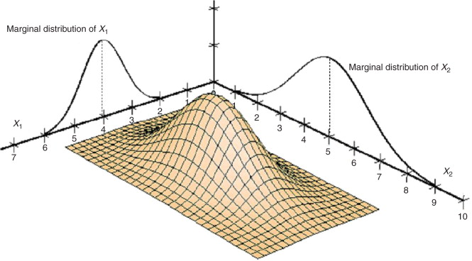
Marginal Probability
For notational clarity, we will use continuous, bivariate distributions to illustrate the remaining concepts. They generalize clearly to the discrete and general multivariate cases.
TLDR: Squishing an entire multivariate distribution into one dimension yields a marginal distribution.
A multivariate PDF completely describes how probability densities change as we move through every dimension of the input space simultaneously. Thus, we can see how different dimensions of the distribution interact. However, we may wish to understand how probability density is distributed over a single dimension; this is more high-level and doesn't give full detail for the distribution. This involves "squashing" the rest of the dimensions into a single-variable distribution over the single dimension (stilted wording).
Let \(X\) and \(Y\) be continuous RVs with joint density function \(f(x,y)\). The marginal density functions of \(X\) and \(Y\) are \(f_X(x)=\displaystyle\displaystyle\int_{-\infty}^{\infty}f(x,y) \, \text{d}y\) and \(f_Y(y)=\displaystyle\int_{-\infty}^{\infty}f(x,y) \, \text{d}x\). The marginal density function \(f_X\) of \(X\) is a univariate distribution describing how the density of \(f(x,y)\)across all values of \(Y\) changes as \(X\) changes (and likewise for \(f_Y\)).
Geometrically, we can associate each value \(x_0\) for \(X\) with a slice of the multivariate distribution \(f(x,y)\), corresponding to region where the distribution has \(X\) value \(x_0\). Each slice has an area. The marginal density function \(f_X(x)\) is the distribution of these areas over all the choices of \(x_0\).
By considering the area instead of the entire shape of the slice, we lose information about the other dimensions.
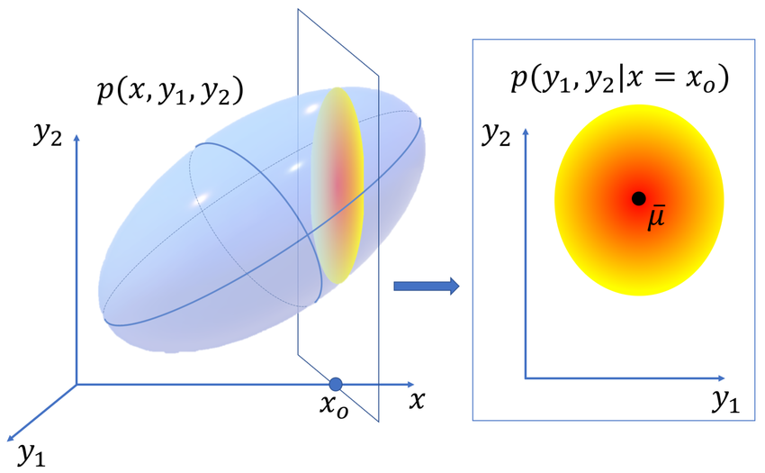
Conditional Density Functions
We may also wish to reason about the distribution of values of \(X\) if we fix a certain \(Y=y_0\). Geometrically, this would be considering the distribution described by the slice of \(f(x,y)\) given by \(f(x,y_0)\) with \(x\in \mathbb{R}\) as a degree of freedom wording. However, the area under this slice might not be \(1\), so we need to normalize the distribution by the slice's area as well.
The conditional density function\(f_{X|Y}\) of \(X\) given \(Y\) is given by \(f_{X|Y}(x\mid y)=\dfrac{f(x,y)}{f_Y(y)}\). So, if we fix \(Y=y_0\) constant, the distribution of values of \(X\) is given by \(f_{X|Y}(x,y_0)=\dfrac{f(x,y_0)}{f_Y(y_0)}\).
Note that the conditional density function is only defined for \(y\) where \(f_Y(y)>0\)
Sometimes we consider the random variable \(X|Y\) directly
Joint Conditional Probabilities
It follows clearly that \(P(X\leq a\mid Y= b)=\displaystyle\int_{-\infty}^{a}f_{X|Y}(x|y=b) \,\text{d}x\) and \(P(X\geq a\mid Y\geq b)=\dfrac{P(X\leq a, Y\leq b)}{P(Y\leq b)}=\dfrac{F(a,b)}{F_Y(b)}\)
When we condition on an equality (e.g. given \(Y=b\)), we are able to simply substitute in the value (here, \(b\)) into the random variable (here, \(Y\)). This gives a univariate function of the other variable over which we integrate.
Independence
We've seen that two events \(A\) and \(B\) are independent when \(P(A\cap B)=P(A)\times P(B)\). We can define the same construct for random variables that comprise a multivariable distribution: random variables \(X\) and \(Y\) are independent when \(f(x,y)=f(x)_X \times f(y)_Y\).
Independence also implies \(f_{X|Y}(x\mid y)=f_X(x)\) and \(f_{Y|X}(y\mid x)=f_Y(y)\)
Formally, we define independence as \(F(x,y)=F_X(x)\times F_Y(y)\) since this covers both the discrete and continuous case. In general, if we want to consider both cases, we use \(F\) and not \(p\) or \(f\).
By corollary, if \(f\) has a rectangular support we are able to factor \(f(x,y)\) into \(g(x)h(y)\) for functions \(g,h\), then \(X\) and \(Y\) are independent and \(g(x)=f_X(x), h(y)=f_Y(y)\). Conversely, if we cannot factor \(f(x,y)\) this way, \(X\) and \(Y\) are dependent. This provides a nice way to show independence without integrating.
Often, \(g,h\) are the recognizable probability density functions of well-known distributions, so looking for these might help us factor \(f(x,y)\).
Why does this only work with a rectangular support? If we require independence, the individual support for each random variable can't change as other random variables change, so it must be a static interval between two constants. Since this is required for all random variables, our support is a product of intervals, a rectangle. Put another way, an irregularly-shaped domain encodes a relationship between different random variables in and of itself, so those variables are not independent.
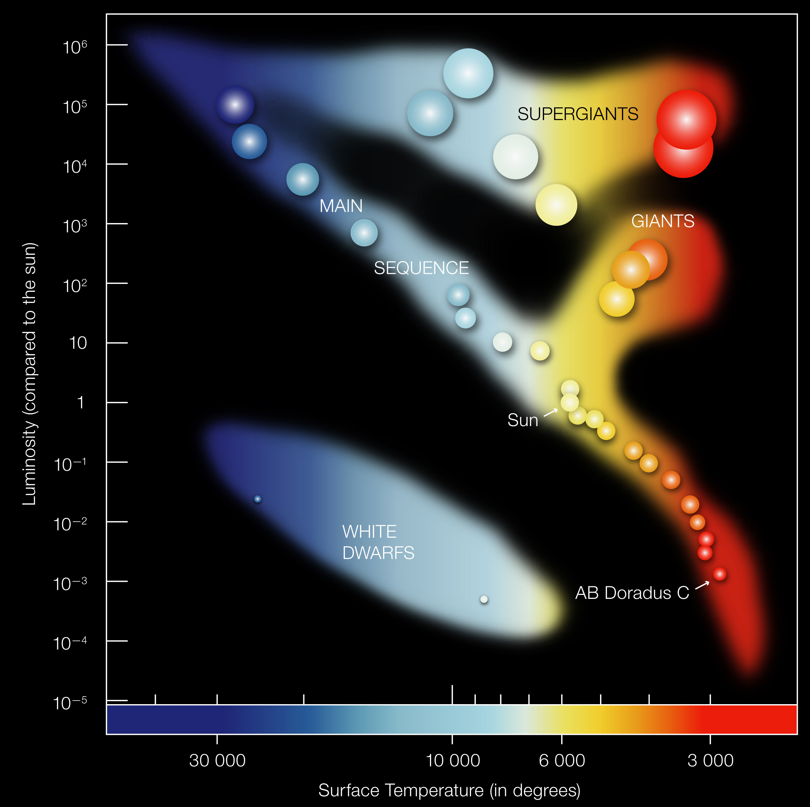
E.g. The usefulness of the HR diagram in astronomy comes not from the density of stars in certain regions, but rather that the support of the joint distribution of star luminosity and color is (extremely) irregular. Much of the information about the relation between these two quantities, which informs what kind of stars exist and how they form, is encoded in the shape of the support.
Expectation and Variance
The multivariate formulation and properties of expectation follow directly from the univariate case. For arbitrary function \(g:S_X\times S_Y\to \mathbb{R}\), we have
Note that because we now have two variables \(x,y\), we need some function \(g:S_X\times S_Y\to \mathbb{R}\) to combine them into a single quantity whose expected value we can reason about
This implies that we can find the expected value of one variable (e.g. \(X\)) using \(g(x,y)=(1)x+(0)y\), yielding the expected (lol) formula
We find the equation for the expectation of a single variable (WLOG, \(X\)) by taking using \(g:(x,y)\mapsto x\). We get \(\mathbb{E}\left[X \right]=\displaystyle \int_{S_X}\int_{S_Y}xf(x,y)\, \text{d}x\,\text{d}y\).
As with before, we have \(V\left[g(X,Y) \right]=\mathbb{E}\left[(g(X,Y))^2 \right]-(\mathbb{E}\left[g(X,Y) \right])^{2}\).
When \(X\) and \(Y\) are independent, we have \(\mathbb{E}\left[h(X)k(Y) \right]=\mathbb{E}\left[h(X) \right] \times \mathbb{E}\left[k(Y) \right]\) where \(h\) is a function depending only on \(X\) and \(k\) is a function depending only on \(Y\).
Note that this does not imply \(\mathbb{E}\left[X^{2} \right]\) is the same as \((\mathbb{E}\left[X \right])^{2}\) because a variable and itself are not independent (in fact, they are as dependent as it is possible to be)
Expectation and variance act the same way as the single-variable case because they are fundamentally single-variable phenomena. Expectation must take one input argument as discussed above. However, variance is the univariate special case of a more general multivariate construct.
Covariance and Correlation
Covariance
It is useful to consider how random variables change. When we have just one variable, all we can really reason about is how much the random variable changes; this is what variance measures. However, with multiple RVs, we can also reason about relationships between changes in multiple random variables. This is related to independence; if independence is a boolean point-estimate, covariance gives us the whole distribution.
The covariance\(\text{Cov}\left[X,Y \right]\) of random variables \(X,Y\) is defined as \(\text{Cov}\left[X,Y \right]=\mathbb{E}\left[(X-\mathbb{E}\left[X \right])(Y-\mathbb{E}\left[Y \right]) \right]\).
We have \(\text{Cov}\left[X,Y \right]=\mathbb{E}\left[XY \right]-\mathbb{E}\left[X \right]\mathbb{E}\left[Y \right]\)
Clearly, variance is a special case of covariance: \(V\left[X \right]=\text{Cov}\left[X,X \right]\)
\(\text{Cov}\left[X,Y \right]\) is \(0\) when (and only when) \(X\) and \(Y\) are independent. In fact, it makes intuitive sense to (mentally) define independence this way, i.e. a covariance of \(0\) is the categorical definition of independence.
This implies that for independent \(X,Y\), we have \(\mathbb{E}\left[XY \right]=\mathbb{E}\left[X \right] \mathbb{E}\left[Y \right]\) since \(\text{Cov}\left[X,Y \right]=0=\mathbb{E}\left[XY \right]-\mathbb{E}\left[X \right]\mathbb{E}\left[Y \right]\), proving what we gave as fact in the previous section
We have the following basic properties:
Covariance of RV and constant is \(0\): \(\text{Cov}\left[c,Y \right]=0\)
Covariance gives us the machinery necessary to reason about the variances of linear combinations (and so, sums) of random variables. If the pairwise covariance between random variables in the sum tends to be high, then the sum itself will have less variance than if all the variables were independent.
We have \(\displaystyle V\left[\sum\limits_{i=1}^{n} a_iX_i \right]=\sum\limits_{i=1}^{n}\sum\limits_{j=1}^{n} a_i a_j \text{Cov}\left[X_i, X_j \right]=\boxed{\sum\limits_{i=1}^{n} a_i ^{2}V\left[X_i \right]+2\sum\limits_{i=1}^{n}\sum\limits_{j=i+1}^{n} a_i a_j \text{Cov}\left[X_i, X_j \right]}\).
There is also a clean formula for the covariance between two different sums of (different) random variables: \(\displaystyle\text{Cov}\left[\sum\limits_{i=1}^{n} a_iX_i, \sum\limits_{j=1}^{m} b_j Y_j \right]=\sum\limits_{i=1}^{n}\sum\limits_{j=1}^{m}a_i b_j \text{Cov}\left[X_i, Y_j \right]\).
Correlation
Covariance measures how much two RVs change together. This is proportional to how similar the behavior of the two variables is, but also to the variances of these variables. To reason directly about how related the behaviours of variables are, we must normalize the covariance by the variances of the variables.
The correlation\(\rho\) of random variables \(X,Y\) is defined as \(\rho=\dfrac{\text{Cov}\left[X,Y \right]}{\sqrt{V\left[X \right]V\left[Y \right]}}=\dfrac{\text{Cov}\left[X,Y \right]}{\sigma_X \sigma_Y}\). Since it is normalized, we always have \(-1\leq \rho\leq 1\) and \(\rho=0\) for independent \(X,Y\).
Conditional Expectation and Variance
The conditional expectation of \(Y\) (and generally, \(g(Y)\)) given that \(X=x_0\) is defined as \(\mathbb{E}\left[g(Y)\mid X=x_0 \right]=\displaystyle \displaystyle\int_{-\infty}^{\infty}g(y)f(y\mid X=x_0) \, \text{d}y\) when \(X\) and \(Y\) are jointly continuous.
In the discrete case, \(\mathbb{E}\left[g(Y)\mid X=x_0 \right]= \displaystyle\sum\limits_{S_Y}g(y) p(y\mid X=x_0)\)
Here, \(f(y\mid X=x_0) \, \text{d}y\) and \(p(y\mid X=x_0) \, \text{d}y\) are just the conditional density functions with the \(x\) argument replaced with the constant \(x_0\).
The conditional variance of \(g(Y)\) given \(X=x\) is thus \(V\left[g(Y)\mid X=x_0 \right]=\mathbb{E}\left[(g(Y))^{2}\mid X=x_0 \right]-(\mathbb{E}\left[g(Y)\mid X=x_0 \right])^{2}\).
Recall that when \(X\) and \(Y\) are independent, the expectation of one variable does not depend on the other. So, we simply have \(\mathbb{E}\left[g(Y)\mid X=x_0 \right]=\mathbb{E}\left[g(Y) \right]\) and \(V\left[g(Y)\mid X=x_0 \right]=V\left[g(Y) \right]\).
Law of Iterated Expectations
So far, it has been clear from context which random variable is the subject of our expectation, i.e. which variable we sum/integrate over. We will denote this explicitly in the following section for clarity.
Law of Total Expectation
Theorem
For random variables \(X\) and \(Y\), we have \(\mathbb{E}_X\left[X \right]=\mathbb{E}_Y\left[\mathbb{E}_X\left[X\mid Y \right] \right]\)
We can understand and prove the theorem by writing the expectation in sum/integral form. We have \(\mathbb{E}_Y\left[ \mathbb{E}_X\left[X\mid Y \right] \right]=\displaystyle \displaystyle\int_{-\infty}^{\infty}\mathbb{E}_X\left[ X\mid Y=y\right] \times p(y) \, \text{d}y=\displaystyle\int_{-\infty}^{\infty} \mathbb{E}\left[X \right] \, \text{d}y=\mathbb{E}\left[X \right]\). We saw the integrand had the same form as the law of total expectation; we see that the law of iterated expectations is the law of total expectation in general form.
By extension, \(\mathbb{E}\left[g(X) \right]=\mathbb{E}\left[\mathbb{E}\left[g(X) \mid Y\right] \right]\)
Aside: I find this statement written in closed form to be unintuitive and difficult to wrap my head around. It makes much more sense when I think about it in its summation/integration form.
It follows that \(V[X]=\mathbb{E}\left[V[X\mid Y] \right] + V\left[\mathbb{E}\left[X\mid Y \right] \right]\)
 ??
??