Lecture 01 - Introduction to Functional Programming
Basic Computer Architecture
Computer model: processor talks to the RAM (take CMPUT 229 for a whole semester worth of this being explained!)
Usually, we load the compiled program into RAM and execute it
Data can be stored to a location, changed, and "deleted" (overwritten)
Requires the idea of an assignment statement
What Does the Program Look like Mid-execution?
Program State
At every phase of its execution, a program has state
Aside: can this be described as a subset of the cartesian product of all of the variables in the program
Side effects: who changed the state?
Updating State
Unstructured programs use global variables that allow uncontrolled access to state
Aside: can this abstract all state management mechanism
Modern language encapsulate access, e.g. with objects
Functional programming is stateless
All about state transition
Each instruction/step in the program may change the state
Programming Paradigms
Originally, programming was done in a assembly, but high-level languages became widely used, so having really good compilers became important
High-level languages provide abstraction over the hardware, and may follow different paradigms
Basic, Fortran: Some of the First
Still around (aaaaaa!!); in-use in older software
Basics has no loops; everything was done with gotos (229 throwback)
Structure of programs is more similar to assembly than more modern languages
Aside: loops and recursion are the basic powerful constructs that help us do things, and are two sides of the same coin
Aside: is it possible to generalize loops, conditionals, goto, etc beyond "loop branches back and if branches forward"?
Imperative: Algol → Pascal → C
More powerful and abstract over hardware
Still tied into the Processor ←→ RAM architecture
Object-oriented: Smalltalk, Java, C++, Python
Object-oriented → everything is done through objects
Developed because greater organization is needed for large projects that purely imperative programming cannot provide
The user of a class should not know (or need to know) how you implemented a class; they just need to use the interface for the implementation that you provide and trust it does what it guarantees
Aside: similar approach as loop invariant is to program verification
Functional: Lisp, Various Others
We use mathematical concepts and structuring to solve programs: describe it in terms of functions!
This will be studied at length in this course
No variables representing memory or assignments
Everything is done by defining functions
Recursion is the main mechanism to do things
Code tends to be terse, with precise meaning
Uses the lambda calculus
Logical: Prolog, Answer Set Programming
A subset of logical language can be used as a programming language
Based on logical deduction
We tell the computer what to do instead of explaining how to do it
Aside: declarative vs. imperative divide
Example use: graph colouring (used to develop cases for four-colour theorem)
Program Concepts
Syntax: how do we write them?
Formal: which texts form valid programs?
Semantics: what does our program mean?
Execution: what does the program actually do when rn?
Fun - A Simple Functional Language
A program is a collection of functions definitions
Functions are defined over lists and atoms
Aside: can atoms be abstracted away as constant functions → maybe?
Computation done by evaluating functions on given arguments
Syntax Terminology and Interpreters
f(x, y) = x * x + y
\(=\) is read as "is defined as"
We can apply a function by replacing sides defined as equal
Can be done for any possible values of \(x\) and \(y\) when the function is applied, i.e. \(\forall x \forall y, f(x, y) = x * x + y\)
Lefthand side: \(f(x, y)\)
Righthand side: \(x * x + y\)
An interpreter needs to (aside: can only?) do two things
Replace a function with its definition (lefthand → righthand)
Substitute variables with arguments provided to the function
Notice that we do not declare types; the programming is responsible for making sure the types are correct
Functions
Function: mapping \(f : A \to B\) from domain (\(A\)) to co-domain (\(B\))
Function definition: what a function does, e.g. \(f : x \mapsto x^2\) (pure) or \(\text{f prints "Hello world" to the standard output}\) (side-effect)
Aside: might be better to refer to pure functions as "functions" and impure functions as "methods" or "procedures"
Function application: evaluation of the function for specific arguments
Total functions are defined over their whole domain
Partial functions are not
Function compositions: for \(f : A \to B\) and \(g : C\supseteq B \to D\), \(g(f(x)) = g \circ f : A \to D\)
Higher-order Functions
Regular functions work on "atomic" data, but higher-order functions may input or output functions themselves
E.g. \(\circ\) is a higher-order function: \(\circ : (A \to B) \times (C \to D) \to (A \to D)\) (woah!)
Function composition enables concise and generic code
Aside: what other things (?) can be expressed like this? can every function/construct?
Aside: can all constructors/operators(?) be conceptualized this way? is this what they have to be?
Types of Objects
Atoms: primitive, inseparable values, including integers and real numbers
Can be literals (numbers, characters, symbols etc) or identifiers (symbols representing a value)
The smallest unit of the program → cannot be split
The symbol atom is a sort of immutable string that exists is a sort of "runtime-level identifier": they are directly comparable in \(O(1)\)
Aside: we can think of symbols as entries in a global enum
Aside: does it make sense as a language feature to have namespaces for symbols? or does this defeat the whole purpose? Philosophically, what are symbols for?
Aside: symbols and enums are two sides of the same coin: we can think of an enum type as the union type of a bunch of symbols
Lists: defined inductively
Empty list \(()\)
If \(x_1 \dots x_n\) are lists of atoms, then \((x_1 \dots x_n)\) is also a list
Nothing else is a list
Defn allows for arbitrary nesting → we can represent leaf-only trees with lists of lists where nested list depth ←→ tree depth
Lists in programming stems from the need to represent our knowledge in terms of symbols
We use these to represent every type of data
Primitive Functions on Lists
We only need three primitive functions to fully manipulate the lists (aside: is there a generalizable reason that just these three are necessary?)
The second element can be empty → inserting the first element of the list
Any nested list can be constructed with cons
E.g. (a, (b)) = cons(a, cons(cons(b, () ), () ) )
Other Primitive Functions
Although we can now define any function with these, in practice, we "need" more functions to make "regular programming" easier
What we have already is enough to build a Turing machine → we can simulate any function (in theory)
Useful primitives
Arithmetic operations: \(+, -, *, /\)
Comparison: \(<, >\)
if, then, and else for conditionals
null(x): true if x is an empty list, false otherwise
equality for atoms eq(x, y)
check if something is an atom atom(x)
Aside: what are all the possible such classes of functions in a programming language, and can any of these primitives be implemented with others? what is the minimal set(s)?
Writing Simple Programs
count(L) returns the number of elements in L, assuming L is a list
count(L) =
    if null(L) then 0
    else 1 + count(r(L))
The program consists of a
Function definition of count(L)
Base case: L is empty, so its length is \(0\)
Recursive case: length is one plus the length of the rest of the list
Aside: a basic model for computation: simple recursive function, analogous to while-loop
Base case → loop condition is satisfied
Recursive case → loop continue condition (condition false)
The evaluation of a program can be traced by performing each substitution step manually
Lecture 02 - Working with Lists
Abstract data type: defining a data type by expressing invariants and desired operations mathematically
E.g. stack pop: \(S_{\text{rest}} \cup {\text{top}} \to S_\text{rest}\)
Framework for abstracting over primitive functions
Implementing Simple List Functions
Member
member(x, L) (abbreviated m)
L is a flat list, x is an atom → simple recursive search
Nested search → recurse if list, check equality if atom (multiple dispatch)
Append
// list[any_1] list[any_2] -> list[any_1 | any_2]

app(L1, L2) =
    if null(L1) then L2
    else app(rmlast L1, cons(last L1), L2)

rmlast(L) =
    if null(rest(L)) then first(L)
Binary Tree
Binary Tree data structure: a tree where each node has 0, 1, or 2 elements
Nodes can be read, inserted, and removed from the tree
Main considerations
Decide how to represent the data structure with lists
Implement an abstract data type for binary trees and their operations as a set of mathematical functions
The user interacts with the data structure with the functions, and shouldn't see the details of our data representation
Lecture 03 - LISP Language Constructs
Two selectors and one constructor allow us to construct and manipulate any list-like structure made with nodes
Accessing List Items
Any element of the list can be accessed by composing two functions
First element: car (equivalent to first)
Rest of the list: cdr (equivalent to rest)
Functions in LISP
The leftmost term in an s-expression is interpreted as a function that gets applied with the rest of the terms as parameters
This first term can either be a primitive function, or a value that evaluates to a function
First-class functions: it is possible to write expressions that evaluate to functions
Functions are defined using defun (define function)
(defun fun_name (params...) (body...))
Functions are defined by name and by their number of parameters (arity)
Function Examples
Top-down strategy for writing functions: write a general implementation of a function that may use helper functions, then implement those helper functions, then theirs, etc.
Creates one or many local bindings within the body of the let expression
Local binding: a value is bound to an identifier in a constant way, i.e. x represents 3
The new bindings are in scope inside of the let expression
Expressions can access the scopes of any let body they are in → nested let expressions allow access to multiple (nested) scopes at the same time
If a deeply nested scope binds an identifier already bound in one of its ancestors, the innermost binding is used, i.e. the most specific scope is preferred
The identifier in this case is re-bound; this is not the same as reassigning its value
let* is a recursive version of let where the identifier representing an expression can be accessed within it
Use case: replacing a long expression used in any places with an identifier (also caches that evaluation)
Aside: functions assigning arguments to their parameters when the function is applied is an example of a local binding (it turns out this is used to implement let itself)
Aside: many languages use {} to denote block scoping; let is essentially the LISP equivalent to that
Equality in LISP
The eq function checks equality between atoms
The equal function can check equality between values of any data type, including lists and s-expressions
List of predicates and expressions after them; if the predicate evaluates to true, we evaluate the expression(s) after it. Otherwise, we move to the next clause
Often, we just have one expression without the implicit begin
Should end with a default case where the predicate is just T
if
(if P1 e2 e3)
Evaluate the predicate P1. If it's true, evaluate to e1, otherwise e3
Equivalent to a cond expression one predicate clause and a default clause
Lecture 04 - S-expressions
Symbolic Expression (s-expression): a generalization of atoms and lists that serves as the "universal" LISP data structure
Recursive definition
An atom is an s-expression
If \(x_1 \dots x_n\) are expressions, then the list \((x_1 \dots x_n)\) is an s-expression
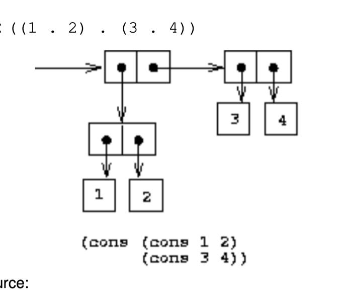
If \(x_1\) and \(x_2\) are s-expressions, then the dotted pair\((x_1 . x_2)\) are s-expressions
Dotted Pairs
Dotted pair: expression formed by combining two non-list values
Think of a "box" with two "cells" that contain pointers to s-exps, whose values can be accessed with car and cdr
Exposes the true, generalized nature of cons
The dotted pair is the, unique way to combine/structure data in LISP
Everything in LISP is stored this way
(car (x . y)) -> x
(cdr (x . y)) -> y
Some dotted pairs are identical to some lists, i.e. if their cars and cdrs are the same
Machine-level Representation
S-expressions in LISP can be one of two things:
Atoms
Dotted pairs
So, anything that isn't an atom is constructed with dotted pairs
A list is a dotted pair where the second cell is a list (possibly empty)
A tree is a dotted pair where both elements are (or have) lists
Simplest Form
Representation with the least amount of dots
Generally, we can simplify/eliminate
Dots . followed by open parentheses(
Matching open/closed parentheses
Many different s-exps may have the same simplest form, and are thus the same
Storing Function Definitions
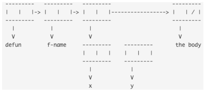
Like any other s-exp, function definitions can be stored as dotted pairs
Symbolic Expression (s-expression): a generalization of atoms and lists that serves as the "universal" LISP data structure
Recursive definition:
An atom is an s-expression
If \(x_1 \dots x_n\) are expressions, then the list\((x_1 \dots x_n)\) is an s-expression
If \(x_1\) and \(x_2\) are s-expressions, then the dotted pair\((x_1 . x_2)\) are s-expressions
Dotted Pairs
Dotted pair: expression formed by combining two non-list values
Think of a "box" with two "cells" that contain pointers to s-exps, whose values can be accessed with car and cdr
Exposes the true, generalized nature of cons
The dotted pair is the, unique way to combine/structure data in LISP
Everything in LISP is stored this way
Aside: lists in LISP are an abstraction over dotted pairs chained together
; IDENTITIES: DOTTED PAIRS

(car (x . y)) -> x
(cdr (x . y)) -> y
Some dotted pairs are identical to some lists, i.e. if their cars and cdrs are the same
E.g. (a . nil) is the same (a)
Machine-level Representation
S-expressions in LISP can be one of two things:
Atoms
Dotted pairs
So, anything that isn't an atom is constructed with dotted pairs
E.g. A list is a dotted pair where the second cell is a list (possibly empty), i.e. a linear chain
Thus, lists in LISP are demonstrably linked lists
E.g. A tree is a dotted pair where both elements are (or have) lists
E.g. A function is a list of its name, parameters, body, etc (more on this later)
Aside: can every possible data structure in LISP be abstracted/generalized as one of the \(2\times 2\) ways to place atoms and lists in a dotted pair structure?
Simplest Form
Simplest form: Representation with the least amount of dots
Aside: we can see list as a function that prints an s-expression in its simplest form
Aside: is a list always the simplest form of an expression
Aside: simplest form is more about a visual representation for us; the machine representation never changes
(a . (b c)) ; example s-expression

; Full dotted-pair form
(a . (b . (c . nil)))

; simplest form
(a b c)
Generally, we can simplify/eliminate
Dots . followed by open parentheses(
Justification: this is the "list nesting mechanism", so we can just represent this part as a list
Matching open/closed parentheses
Many different s-exps may have the same simplest form, and are thus the same (this is an equality test)
Storing Function Definitions
Like any other s-exp, function definitions can be stored as dotted pairs
Dot syntax: represents car and cdr in list notation, but doesn't require writing it out
(1 . (2 . (3 . nil))) corresponds to (list 1 2 3)
(a . b) stands for a cons cell whose car is the object a and whose cdr is the object b
Essentially a shortened, infix cons?
Use case: makes it easier than regular list or ' syntax to declare lists with non-nil terminator
Regular list syntax automatically assumes your list ends with nil
Some dotted pairs are identical to some lists
If a cdr points to an atom, we cannot avoid using a dot (unless we write everything with cons)
If there are no dots, then the list is a proper list
Generalizing the Idea of cons
We have been thinking of cons as a list constructor, but it is more general than that
cons is a "cell" that contains
car: a pointer to something
cdr: another pointer to something (often another list)
Symbolic Expressions (s-expressions)
Symbolic expressions are a generalization of the expressions that can be in the lisp language
It is defined recursively
An atom is an s-expression (base case)
If \(x_1 \dots x_n\) are s-expressions, then \((x_1, \dots, x_n)\) is an s-expression
If \(x_1, x_2\) are s-expressions, then \((x_1 . x_2)\) is an s-expression
Func. Ion Definitions
Stored like any other s-expression
Makes it easy to write higher order functions, which input and/or output other functions
Lecture 06 - Higher Order Functions
Higher-order Functions
Software development tip: don't repeat yourself (DRY);
Can be done with higher-order functions by separating a computation pattern from the specific action
E.g. the pattern of iterating over a list and doing something to each element.
Without higher-order functions, any code doing this would have to be rewritten with a different action hard-coded in
With higher-order functions, the function to apply can be passed in as a parameter to a function (here, map) that applies it to each element
Common Higher-order Functions
Map: apply the given function to every element in the list to get a new list
; map: T[n], (T -> S) -> S[n]
Separates the iteration over the list (generalized with map) and the action done on each element (left as parameter, function to do this provided as argument)
Aside: mapcar and mapcdr exist and are useful in LISP
Aside: map generalizes "structural recursion", i.e. when you join the current value and recursive call with cons to preserve the structure you are recursing over
; reduce call
(map (lambda (x) (x-body...)) L)

; ; equivalent structural-recusive function (sketch, no base case)
(defun rec-fun (L)
    (cons ((lambda (x) (x-body...)) (car L)) (rec-fun (cdr L))))
Reduce: combine elements of a list pairwise until they reduce to a non (or less nested) list
; reduce: T[n], ((T, T) -> T) -> T
The function's identity element may be provided; applying the identity and another argument should return that argument (e.g. if the operation is \(\times\), identity is \(1\))
However, most implementations (conveniently) stop the reduction after applying the reduction function on the last two elements, instead of the last element and the identity
Aside: algebra time 😎
Aside: Reduce can be implemented left or right associatively, i.e. accumulated result is the first or second argument in the function
Also known as fold-left/fold-right
Aside: reduce (left) abstracts tail-recursion in the same way that map abstracts iteration (i.e. recursion with cons connecting the recursive case)
So, if you use cons as the reduction function, you get map
; reduce call
(reduce (lambda (x y) (xy-body...)) L)

; equivalent tail-recusive function (sketch, no base case)
(defun rec-fun (L)
    ((lambda (x y) (xy-body...)) (car L) (rec-fun (cdr L))))
Mapreduce: a map followed by a reduction
This operation is often used in the real world (e.g. querying DBs), so a specific implementation for mapreduce may be more efficient then simply composing map and reduce
Filter: uses a predicate function to remove elements from the list that the predicate finds false
; filter: T[n], (T -> boolean) -> T[m <= n]
Aside: LISP's "filter" functions are named remove-if and remove-if-not
First-class Functions as a Language Feature
Most languages have some syntactic barrier between regular variable use and function application that makes them easy to identify; LISP does not have this at the syntax level
I.e. function applications "look like" using variables
Builtin functions and LISP: apply and funcall apply functions from lists of arguments
Difference: apply takes a list of arguments, funcall takes them as parameters. They are syntactic sugar over the same functionality
Aside: this is an explicit instruction to LISP that a function is being applied; not fancy parsing is necessary
Aside: are regular function applications syntactic sugar over this, or are these syntactic sugar over regular applications?
Aside: what are the implications of abstracting function application as a function itself?
Lecture 07 - λ Calculus I
[[lambda-cal.pdf]]
[[lambda-reductions.pdf]]
At first, computers just did numerical computation, like one would on a (fancy) calculator
Later, we extended computation to include the manipulation of symbols, i.e. programming
Aside: in pure functional programming, any/every computation is a (complex) nested succession of function applications
Since lisp is an early language, its λ calculus implementation is a bit awkward
Lambda Calculus
Aside: \(\lambda\) is the best greek letter, fight me
Pure lisp is already small (in terms of number of primitives), but the lambda calculus is even smaller
The lambda calculus is a minimal but complete model of computation (!)
Similar in ideal to how a Turing machine is a conceptually simple model of complete computation
Motivation/Derivation: get rid of named functions: everything is anonymous functions
Lambda Functions
Lambda functions are anonymous functions, i.e. functions that are not bound to an identifier
Aside: in LISP, function definitions are just syntactic sugar (?) over binding a lambda function to a name in a let expression
Aside: naming functions makes things much easier to keep track of in programs, but these can all be substituted in for anonymous functions without difference
Defining a lambda function is same process as using a literal like 2 or 'a somewhere in a program without binding it
Aside: this is a design pattern called left-left-lambda
Lambda functions can also be called with arguments with funcall and apply
Aside: A closure is generated when a lambda function is defined; when the function is applied, that closure information is fetched and used (more on this later)
Internal Representation
The function function in LISP takes a lambda expression and returns an internal representation of that definition
; function function application
(function (lambda (x) (+ x 1)))

; result
#<FUNCTION (LAMBDA (X)) {11EAF6E5}>
Aside: what LISP language construct is #<...>?
Aside: how is a function body "hashed", like in this example?
Syntax of the Lambda Calculus
The lambda calculus is a minimal, abstract formal language/model of computation with only four constructs
Aside: in terms of programming language design, we can think of this as being the simple possible set of core language features; we can create the rest of the language concepts using syntactic sugar
Aside: the syntax of programming languages (and other similar, complicated concepts) are most elegantly and succinctly described through mutual recursion; analyzing the structure of this recursion yields insights on how the language works
Mutual recursion between function and expression
Mutual recursion between expression and application
identifier is not recursive: implies all λ calculus programs consist of identifiers and syntax
Different "cases" of (possibly mutual) recursion apply to different "language concepts", i.e. in expression, nested functions (application case) and higher order functions (function case)
Aside: is there a way to formally define and generalize "language concepts" by analyzing this "recursion graph"? Are "recursion graphs" a thing (aside: this graph is cyclic iff recursion)
Currying
An \(n\)-ary function can be defined in terms of unary (higher-order) functions; this procedure is currying
Aside: It is a "reverse abstraction" for multivariate functions
; greater than function
; no currying
(lambda (x y) (> x y))
; curried version
(lambda (x) (lambda (y) (> x y)))

; curried application
; aruments: arg-x, arg-y
((lambda (x) ((lambda (y) (> x y)) arg-y)) arg-x)
Uses the property that applying a function binds parameters to arguments in the scope of the function body
The "parameters" that aren't defined in the current lambda function are "hardcoded" into the function definition by virtue of being defined in the scope of the definition of the new lambda function
Procedure
We if have a function \(f : X \times Y \times Z \to D\), we "split" it into \(f : X \to (Y \times Z \to D)\), where \((Y \times Z \to D)\) is a function mapping \(Y \times Z \to D\).
Now, we have a function with one argument that maps to a function with two arguments, which in turn maps to one argument
We keep on "splitting" this second function until all the fns have one argument: \(f : X \to Y \to Z \to D\)
Our function application now looks like \(f(x)(y)(z)\) instead of \(f(x, y, z)\)
Application
Applying a curried function will lead to a set of nested funcall, function, and lambda expressions for each parameter
Example here [[lambda-cal.pdf]]
Reductions in Lambda Calculus
[[lambda-example.pdf|Lambda Reduction Examples]]
A reduction is a step in the process of evaluating an expression
In Lambda Calculus, all reductions happen in lambda expressions, since the syntax consists only of these and (irreducible) atoms
Operational semantics: the process and underlying idea of reducing the language to a value
In Lambda Calculus, this is done with substitutions
LC does not need built-in primitive functions and atoms; they can all be constructed (e.g. \(\mathbb{N}\))
This is non-trivial, but possible
CS 245 / CMPUT 272 flashback!!
Beta-reduction
Beta (\(\beta\)) reduction: given an expression, replace all occurrences of parameters with the argument specified
Equivalent to function application and eager evaluation
; LISP expression
((lambda (x) (+ x 1)) a)
; beta-reduced LISP expression
(+ a 1)
Reductions may actually lead to more complex expressions (i.e. replacing an identifier with a long expression many times in a function definition), so reduction is unstable, and a simplest form is not guaranteed
Alpha-reduction
Alpha (\(\alpha\)) reduction: renaming a variable that is already bound
Changing the name of bound variables doesn't affect computation
We want to assure that a naming conflict does not happen
Aside: choosing names to avoid conflict is called hygiene
Free and Bound Variables
A bound variable is defined in the local scope; a free variable is not
"free" and "bound" are not absolute; they depend on the scope
Thus, changing the names of free variables may cause naming conflicts, since we don't know what naming conflicts exist in the superscope. Thus, renaming a free variable to a bound one could lead to a naming conflict
Global variables are bound in every scope, including the top-level (global) one
Beta vs. Alpha Use-case
We need alpha reduction for cases when direct reduction fails due to naming conflict:
((lambda (x) (lambda (z) (x z))) z); both a bound z in the lambdas and a free z as a parameter
Notice if we blindly use beta-reduction, we get
; direct substitution without renaming((lambda (x) (lambda (z) (x z))) z); sub x -> z(lambda (z) (z z)); naming conflict! big L!
Reduction use: we use alpha reduction to rename bound variables in the local scope that conflict with superscope variables, then use beta reduction to evaluate the functions
This is known as correct beta-reduction
Aside: we can prove functions are different by beta-reducing them, since reduction (by definition) preserves the meaning/result (semantics?) of the function
Lambda Normal Form
A lambda expression that cannot be further reduced by beta reduction is in normal form
Not all lambda expressions can be reduced to a normal form; sometimes the reduction forms an infinite loop.
E.g. ((lambda (x) (x x)) (lambda (z) (z z))) does not have a normal form; doing \(\alpha\) then \(\beta\) substitution yields the same function
Aside: do we prove irreducibility by showing that a reduction leads to a value already found in the "reduction chain"?
Aside: there are other examples of expressions that keep expanding as well; types of these expressions are essential for encoding recursive functions (e.g. the Y combinator)
Lecture 08 - λ Calculus II, Electric Boogaloo
[[lambda-reductions.pdf]]
Lambda Calculus Cont.
Order of Reduction
In which order should we reduce nested function applications?
Aside: this is a fundamental choice one can make while designing a programming language
Generally, the leftmost function needing reduction is reduced first
Normal Order Reduction (NOR)
Normal Order Reduction (NOR): evaluate the leftmost outermost function application
I.e. evaluate the outer function, only evaluate the arguments when you need to
Known as lazy evaluation
f(g(2)) -> g(2) + g(2) -> 3 + g(2) -> 3 + 3 -> 6
May terminate in cases are AOR does not, i.e. an infinitely recursive function nested inside a constant function (since the constant function is evaluated first)
Applicative Order Reduction (AOR)
Applicative Order Reduction (AOR): evaluate the leftmost innermost function application
I.e. evaluate arguments before function
Known as eager evaluation
Most programming languages evaluate this way
Aside: is the reason only functional programming languages have non-eager evaluation because of pure-functional languages having no side-effects? How can this idea be expressed formally?
f(g(2)) -> f(3) -> 3 + 3 -> 6
Is generally more efficient; note that \(g(2)\) is evaluated once under AOR, but twice under NOR
Church-Rosser Theorem
Church-Rosser Theorem
Theorem
If \(A \to B\) and \(A \to C\), then there exists an expression \(D\) such that \(B \to D\) and \(C \to D\)
True even if \(A\)doesn't have a normal form
If \(A\) has a normal form\(E\), then there is a normal order reduction\(A \to E\)
where \(\to\) means a sequence of \(0\) or more reduction steps
NOR guarantees termination if the given expression has a normal form
Aside: Church-Rosser doesn't indicate whether a normal form exists or how many steps we would need to find it; that question is undecidable (its reducibility to the halting problem is evident)
Programming is tied to representation; a problem is given in one form, and our responsibility is to encode into a different form that the computer can interpret
All primitive functions are syntactic sugar over the lambda calculus (or another model)
Natural Numbers
Natural numbers are recursively built from \(0\) by the successor function\(s(n)\); we have \(s : n \mapsto n+1\), so any natural number can be represented by \(n\) nested \(s(n)\) functions around \(0\)
Numeric ("shorthand")
Symbolic
Functional
\(0\)
\(0\)
\((λsx\mid x)\)
\(1\)
\(s(0)\)
\((λsx\mid sx)\)
\(2\)
\(s(s(0))\)
\((λsx\mid s(sx))\)
…
…
…
\(n\)
\(s(\dots s(0)\dots)\)
\((λsx\mid s(\dots(sx)\dots))\)
\(n \in \mathbb{N}\) represented functionally the anonymous (lambda) function that takes the successor function \(s\) and a "dummy parameter" \(x\) as parameters, and nests \(s\)\(n\) times around \(x\)
This function isn't meant to be applied; it represents the number in an of itself.
Thus, the successor function in lambda calculus is SUC: s = (λxsz | s(xsz)), where z is the parameter representing the number whose successor we are trying to compute.
Aside: formally, a successor function\(S : \mathbb{N}\to \mathbb{N}\) is any function with the following properties
For all \(x\in \mathbb{N}\), \(S(x) \ne x\)
\(S\) is one-to-one, i.e. \(S(x) = S(y) \implies x=y\)
There exists some \(e \in \mathbb{N}\) such that, for all \(x \in \mathbb{N}\), \(S(x) \ne e\)
Aside: is this function unique?
Addition
We can implement addition with the successor function:
ADD = (λwzsx | ws(zsx))
Here, w and z represent the numbers we are adding
Performing this reduction manually reveals that this applies the successor s function to zw times, i.e. performing the repeated \(+1\) that defines addition
Control Flow
Conditionals and control flow can be implemented by defining two truth values (true/false) as functional expressions, then choosing control flow based on the outcome of a boolean expression
Aside: this ties into boolean algebras, since "two truth values" (and logical connectives, it turns out) are abstracted by boolean algebras
T = (λxy | x)
F = (λxy | y)

IF = (λxyz | xyz)
Here, we're defining true or false as functions that return either their first or second arguments, and IF simply applies its arguments to the given function (boolean value)
Aside: it seems like values (e.g. T, F, etc.) are defined as simple, non-recursive lambda-expressions, whereas functions (eg. ADD are defined as recursive ones)
Aside: is there something in the function definition of IF that makes it "control flow", different from just a "function"? Of course, assembly indicates how control flows can be explained as jumps backward/forward, etc. There's lots of asides here, more in the [[Autopsy - Asides!|Assignment 2 (Interpreter) Autopsy]]
Logical Connectives
Having defined T and F, we can define logical connectives like NOT, AND, and OR as well
NOT = (λx | xFT)

AND = (λxy | xyF)
OR = (λxy | xTy)
Aside: it is clear that the structure of the function bodies of AND and OR mirrors the "reduction rules" for and and or in racket explained in CS 135
Aside: is there something that makes and and or "fundamental" in logic that is apparent when they are expressed this way?
Aside: can all \(2^{2^{2}}= 16\) logical connectives be expressed this way, i.e. as a simple string of x, y, and T|F? (I don't think it can). What does it mean if a connective can't? Are all combinations of these valid connectives?
Aside: it's interesting how these definitions encode the "trueness" of OR and "falseness" of AND, almost like "default values" if no arguments are provided (once again, like the racket reduction rules). Most rigorous CS student logic.
Boolean Functions
E.g. ZEROT, which test if a value is \(0\)
Aside: these granular functions seem quite similar to the assembly instructions that "build up" all of imperative programming. Is there a minimal set of those? And why are those connections there, even though the models of computation involved are very different? Do all computational models share similarities? (later note: SECD machine answers this a bit)
ZEROT = (λx | x F NOT F)
If x is anything other than the function representing \(0\), the function representing the number will not "throw out" the first F, leading to a negation of NOT F → F
Aside: these definitions of functions are incredibly interesting; I should look up more
Recursion, Generalized
Foundationally, recursion is a mechanism that can execute the same code repeatedly, with possibly different parameter values
Aside: won't parameter values always be different, or an infinite loop occurs (in a pure functional language)?
Thus, we need to create a lambda expression that can produce its argument repeatedly
Combinators
All recursive functions can be defined in terms of a few functions, called combinators
Aside: !!!!!!!!!!!!!
Aside: again, analogy to any program being expressible by ~12 assembly instructions
The Y-combinator generates an arbitrary amount of copies of the expression it is applied to
Aside: the Y-combinator generalizes recursion by allowing a function to "call" (really, replicate) itself without referring to its own name
// DEFINITION
Y = (λy | (λx|y(xx)) (λx|y(xx)))

// APPLICATION
Y N = (Ly | (Lx|y(xx)) (Lx|y(xx))) N
      -> (Lx|N(xx)) (Lx|N(xx)))
      -> N ((Lx|N(xx)) (Lx|N(xx)))
      -> N (N ((Lx|N(xx)) (Lx|N(xx))))
      ...
More (notationally) conveniently, we get N(YN) → N(N(YN)) → N(N(N(YN))), etc
NOR must be applied on the reduction for it to terminate
Aside: this seems to be true of recursion in general; I think this is why functions used for recursion are defined weirdly, i.e. if doesn't evaluate all its arguments and and and or are short-circuitable
Lecture 09 - Context and Closure
[[context-based-intepreter.pdf]]
Our regular reduction strategy is inefficient; we can improve reduction efficiency by deferring the evaluation of expressions until we need them, which is achieved using context and closure
This is known as deferred evaluation or lazy evaluation
Aside: almost seems like a queue; values are cached to the expressions they are bound to, and these whole expressions are stored in the context. Then, when the bound value is called, that expression is evaluated, possibly adding more to the context. This seems to be a complete (yet elegant) way to evaluate only what needs to be evaluated
Context and Closure
A context is a list of (current) bindings\(n_1 \to v_1 , \dots, n_k \to v_k\) where \(n_i\) are identifiers and and \(v_i\) are expressions (note: not necessarily atoms)
The expressions \(v_1 \dots v_k\) may also be closures; these data structures are mutually recursive
A closure is a pair \([\lambda, \text{CT}]\), where \(\lambda\) is a lambda function and \(\text{CT}\) is a (possibly empty) context
When a function is applied, we know its parameters and definition from \(\lambda\), and the values for body variables from \(\text{CT}\)
Closures "close" open (free) variables by binding them to values
Closures result from evaluating lambda functions, i.e. the context gets stored
In LISP, a dotted pair is used to store closures
Functions, including interpreters, need the "current" context to be evaluated properly
Aside: I think we're about to explain that we can pass the current environment as an accumulated stack-like parameter recursively, where new bindings are pushed to the start (which makes nested scoping easy). This seems equivalent to having a global "store" that maps variable names to values, and is mutated. Is it?
Static scope: scope is determined by the structure of the code, i.e. the blocks of the current expression from inner → outer
Dynamic scope: scope is determined by the current state of the environment/store
Deferred Substitution
Substitution is delayed until required using contexts and closures
E.g. λx | (+ x 4)) 2
Old method: we beta-reduce this by substituting x with 2 directly to get (+ 2 4)
New method: we don't change the function body, but we record the bindingx -> 2 in the context
Eval Walkthrough
Evaluation starts with an empty context, since no bindings have been created yet
Aside: In a sense, all syntactic sugar functions in LISP are bindings of their names to function definitions in the global context; global constants are as well. So, the initial context isn't actually empty
When a function is applied,
Its arguments are evaluated in the current context
The function body is evaluated in the current context
The context is extended
Parameter names are bound to arguments (aside: using let?)
The context is extended by adding the new bindings; this forms the new context
Body is evaluated in new context
Asides
Function Application in a Context
Aside: pattern of checking which type of function we are evaluating, then calling whatever we need to (usually the native version of that function): dispatch
Aside: pattern of constructing an expression to evaluate recursively in terms of the language we are interpreting: syntactic sugar/surface syntax
Aside: is this a formal-ish defn of this?
Asides: let
Aside: what is a recursive block? Can a function refer to its own identifier to call itself recursively? Can this be considered a programming language feature? Can other programming features/patterns be generalized/described as this?
Aside: we are using dotted pairs for let; lisp uses lists. Ours is a bit easier to use
Aside: we can write let as a lambda function application; this seems to imply that it's not lambda that has a hidden let statement, but let that has a hidden lambda function. It seems that the generalization flows towards functions, which shouldn't surprise me in a functional language
; let
(let ((x1 e1) ... (xn en)) e)
; lambda function equivalent to let
((lambda (x1 ... xk) e) e1 ... ek)
Lecture 10 - "Interpreter? I barely know her!"
[[context-based-intepreter.pdf]]
Implementing a Context for Our Interpreter
Context data structure: two lists, one of names and one of values, where each pairwise elements correspond (essentially, an association list)
Bindings are added by appending (pushing) to the list with cons and removed by replacing the list with its cdr (popping)
The list is searched left→right to find bindings
This solves the re-binding problem, since the newest binding is leftmost in the list and will be found first. When this gets removed, the old binding still remains! So elegant!
Aside: LISP lists are actually stacks, where cons ⇔ push and cdr ⇔ pop
Aside: this is analogous to the call stack in an imperative runtime model
The eval Function
We will define a function eval to evaluate any s-expression; this is our interpreter
As such, it is not part of the language we wish to interpret
Aside: when should we conceptualize eval as a "regular" function vs. something else?
eval[e, n, v] evaluates expression e in the context defined by name listn and value listv
Like any language-syntax concept, evaluation patterns are recursive; generally, we call eval on the arguments, then defer to the implementation language (and possibly a custom implementation) to interprets the function itself (dispatch pattern)
A helper function evalList that calls eval on each element is useful for evaluating arguments
Evaluation Patterns
Simple Cases
Constants c: just return c
Variables x: look x up in the name list, return the corresponding v in the variable list
Remember, "pushing" to the context when entering a scope assures that most current definition and/or binding of the variable is used
Aside: "pushing" to context and entering a scope are definitionally the same thing, right?
Arithmetic, relational, structural expressions: call eval on all the arguments, then call the corresponding function in LISP (dispatch pattern)
E.g. eval[(⨁ e1 e2), n, v] → eval[e1, v, n] ⨁ eval[e2, n, v]
Conditional expressions: we use the built-in if statements in our implementation language
We always evaluate the condition (first expression)
We don't want to evaluate the part that the conditional doesn't evaluate to, since by definition it won't be used, will reduce performance, and may cause an infinite loop
Aside: this means if isn't a "true function", as established in previous asides
Functions
Lambda functions: evaluate to a closure which contains the function body, variable list, and the context when the function was defined
Parts of a closureC: params(C), body(C), names(C), values(C)
names(C) and values(C) form the context
We can store this in a a pair of dotted pairs, then define accessor functions for them
Function applications: require updating the context and pushing to the stack, since we are evaluating a closure that has its own bindings; we push these onto the stack
We evaluate the body of the closure in the new environment created by appending (with cons) the names and values of the closure to the existing environment
Aside: we have an eval(x) → eval(y) situation, i.e. we call eval again, just with new arguments. This is kinda a different "type" of recursion
Aside: I think this might be the characterization of syntactic sugar; a function is syntactic sugar if and only if it is evaluated by a directly recursive call to the evaluation function using other language constructs
Aside: I stumbled through this implementation before reading this slides (nice!); I learned that an environment system is necessary to implement function applications
C = eval[e, n, v]
z = evalList[(e1 ... ek), n, v]

eval[(e e1 ... ek), n, v] ->

eval[
    body(C),
    cons(params(C), names(C)),
    cons(z, values(C))
]
Scoping
As know, let is a special case of function application where the bindings we define in let become the parameter-argument bindings of the function application, and the body of the let expression is just the body of the function
Aside: a let expression is just a closure, but where the body is defined at evaluation time, almost like being passed as a parameter
Aside: this confirms that let is a type of function definition, as opposed to function applications being surface syntax that use let during desugaring
Evaluating let simply appends the let's bindings to the context, then evaluates the body
Aside: another instance of eval(x) → eval(y) recursion
z = evalList[(e1 ... ek), n, v]

eval[(let (x1.e1) ... (xk.ek) e), n, v] -> eval[e, cons((x1 ... xk), n), cons(z, v)]
Lecture 11 - SECD "Architecture"
[[SECD Machine.pdf]]
Purpose: to execute compiled code on an abstract machine
Think JVM: we compile the program to bytecode, which runs on a virtual machine that maps onto the host machine's instruction set
Thus, we can compile once to bytecode, then compile to whatever assembly language we need. Compilation can also include optimizations as well
The SECD "language" is a language formed of operators, constants, variables (?), and built-in functions, intended as a compilation target for functional languages
The SECD "machine"/"runtime" is a model for executing programs written in the "SECD language" using four stacks
Aside: I wonder how hard this would be to implement as a Turing machine
Execution
Stacks 💸
The SECD machine is built using four stacks
Each stack can be represented by an list s-expression, where the top of the stack is the first element of the list
Asides: this isn't representation, as much as LISP "lists" are stacks
Structure
The evaluation stack is used to evaluate expressions
To perform an operation is to pop elements from \(s\), perform the operation, then put the result back on \(s\)
For unary op, we have \((a.s)\, e\, (\text{OP}.c)\,d \to ((\text{OP} a).s)\, e\, c\, d\)
When evaluation is done recursively, sub-expressions are pushed to this stack each time they are called
Since SECD uses reverse Polish notation, the structure of the recursion is reflected in the stack, so the result of the evaluation of a subexpression will be on the right place in the stack to be used to compute the expression it is a part of
The environment is used to keep track of bindings
Aside: see, I told you environments lend themselves to being stacks!
The control is used to store instructions
In the program's initial state, the entire program is loaded into the control stack, and the rest of the stacks are empty
The dump is used to store suspended invocation context, i.e. eval that we will come back to later
Analogous to the call stack in C-style languages
E.g. when compiling an if-statement, the dump stack is used to store the rest of the control stack while the control inside the chosen if-statement boy is compiled
E.g. when compiling a function application, the whole eval stack, environment, and control stacks are appended to the dump stack, then restored when we return from the function application's scope
Operations
An operation is like an assembly instruction; it is defined in terms of its effect on the four stacks, i.e. \(s\, e\, c\, d\, \to s'\, e'\, c'\, d'\)
Aside: we can think of the state of the program as the state of the four stacks; this makes the operations state transitions/reducers
Aside: operations define reductions, analogous to the reductions we make in lambda calculus
Aside: Just realized why the reducer pattern (common in React.js, for example) is named as it is; due to the link between reduction in things like lambda calculus and thinks like the SECD machine
Aside: reductions can define a sort of "graph structure"; how can we analyze that to gain insights about the reduction/evaluation process?
Reminder: these stacks are formed of dotted pairs; we will use dotted pairs in the definitions (e.g. \((\text{NIL}.s)\) pushes \(\text{NIL}\) to the stack \(s\), since \((\text{NIL}.s)\) is a dotted pair)
OP
Description
Definition
Explanation
NIL
push a nil pointer
\(s \, e\,(\text{NIL.c})\, d \to (\text{NIL}.s)\, e \, c \, d\)
moves a nil pointer from the control stack to the evaluation stack
LD
load from the environment
\(s \, e\,(\text{LD} (i.j).c)\, d \to (\text{locate}((i.j),e).s)\, e \, c \, d\)
uses locate (auxiliary function) to find the value of a variable in the environment
LDC
load constant
\(s \, e\,((\text{LDC} x) .c)\, d \to (x.s)\, e \, c \, d\)
moves a constant from the control stack to the evaluation stack
LDF
load function
\(s \, e\,((\text{LDF} f) .c)\, d \to ((f.e).s)\, e \, c \, d\)
Adds function to eval stack from control stack
AP
apply function
\(((f.e') v.s)\, e\, (AP.c)\, d \to \text{NIL}\, (v.e')\, f\, (s e c.d)\)
applies a function, analogous to a JAL instruction
RTN
return
\((x.z)\, e'\, (\text{RTN}.q)\, (s e c.d) \to (x.s)\, e\, c\, d\)
restores the environment from when the fn was called
SEL
select in if-statement
\((x.s)\, e\,((\text{SEL}\, \text{ct}\, \text{cf}).c)\, d \to s\, e \, c' \, (c.d))\)
delegated to to compile if-statements, since they require special compilation to not execute both paths
used with SEL; adds what was in the dump stack to the control stack
RAP
recursive apply (details omitted)
DUM
create a dummy env
used with RAP
Aside: all the operations "exist" (i.e. written) in the control stack first because the control stack dictates what the next instruction is; by definition, the control stack becomes \(c\) because that instruction is removed
Aside: logically, then, the whole program must be "loaded" into the control stack; the initial state of the program
Aside: how can we abstract away auxiliary functions?
Aside: can all these functions be generalized by which stacks they use? Can any of these be characterized uniquely by that?
Compilation (LISP)
Built-in Functions
Built-in functions: A built-in LISP function (OP e1 ... e2) is compiled to "SECD language" instructions (ek' || ... || e' || (OP))
E.g. (* (+ 6 2) 3) is compiled to (LDC 3 LDC 2 LDC 6 + *)
e1' … ek' are the compiled versions of the LISP expressions e1 … ek
As we have come to expect, the "compile function" is recursive
Here, || indicates appending instructions together
Note the order of compiled expressions is in reverse; this implies that expressions in SECD are written in reverse Polish notation
Aside: RPN is used here because it can be evaluated using a stack structure
If-then-else
If-then-else: the LISP function (if e1 e2 e3) is compiled to e1' || (SEL) || (e2' || (JOIN)) || (e3' || (JOIN))
We are essentially delegating the special if/else logic to SEL; we can't implement an if/else statement that doesn't evaluate both its arguments with functions alone
Aside: does this mean, fundamentally, we need an imperative if (if)? Is that what the "special" if/else fundamentally isn't
Aside: does conditional logic always need to get delegated down the chain of abstraction until it reaches assembly branch instructions?
Aside: how does short-circuiting and and or work here, since they seem to have similar "special" status like if/else, but not a special implementation?
Can we implement short circuiting (only) with a special if/else?
Non-recursive Functions
Lambda Functions: A LISP lambda function (lambda (arg1 ...) (body...)) is compiled to (LDF) || (body' || (RTN))
Here, body' is the compiled body code
RTN represents a "return" instruction, indicating the function is done
Aside: needing to add this is a consequence of doing a functional→imperative transform (compilation)
Function application: A LISP function application (e e1 ... ek) is compiled to (NIL) || ek' || (CONS) || ... || (CONS) || e1' || (CONS) || e' || (AP)
LDF loads a function from the control to the eval stack
AP applies a function by
Saving the state of the \(s\), \(e\), and \(c\) stacks in the dump stack
Setting the eval stack to NIL (since whatever is built up there is outside the function body, and shouldn't affect the function application)
Aside: this is equivalent to jumping to the new place in instruction memory where the function definition is located
Adding the parameter-argument bindings from the function to the environment
Setting the control stack to the function itself
Aside: parallels can be drawn between this and using JAL type instructions in assembly
Scoping (let) statement: A LISP let statement (let (x1 ... xk) (e1 ... ek) exp) is compiled to (NIL) || ek' || (CONS) || ... || e1' || (CONS LDF) || (e' || (RTN)) || (AP)
Notice the similarity to the function application and lambda function code; the semantics of an application and a let expression are essentially the same
Recursive Functions
Recursive functions: the LISP function (letrec (f1 ... fk) (e1 ... ek) exp) is compiled to (DUM NIL) || ek' || (CONS) || ... || e1' || (CONS LDF) || (exp' || (RTN)) || (RAP)
Optional topic: more on that in the [[SECD Machine.pdf|notes]]
Note: Generating Indices for Identifiers
The names of identifiers are compiled away; they are accessed in the environment as numbered indices
These are generated in the order the functions are called (i.e. outermost functions have lower indices), and then by parameter order
So, each identifier is stored as a dotted pair of numbers
E.g. ((lambda (z) ((lambda (x y) (+ (- x y) z)) 3 5)) 6) compiles to (LD (1.1)), (LD (1.2)), (LD (2.1))
Lecture 13 - Intro to Logic Programming through Prolog
In Horn clause logic programming, a program is a collection of Horn clauses of the form \(A \leftarrow B_1, \dots, B_n\), where \(A\) and \(B_i\) are atoms
Computations are deductions in Horn Logic
Prolog
Prolog is a programming language that implements Horn Logic LP.
Prolog is a declarative programming language; facts and rules are declared, and computations are executed by running queries on the facts and rules
Grammar
The syntax of prolog is based on predicate calculus (wikipedia), which is formed of predicates (relations) over non-logical variables
Unlike "real" predicate calculus, prolog doesn't use quantifiers
An atom/atomic formulap(t1, ..., tn) is formed of a predicate symbolp that encodes a predicate (relation) over termst1 ... tn
Aside: note that unlike LISP, "atoms" are relations, i.e. compound structures; this reflects "atomicity" in a logical since (i.e. the predicate as the basic logical unit) as opposed to a syntactic sense. However, atom is not incorrect syntactically, since terms can only be used in predicates
Types of Terms
Constants: numbers (as literals), booleans (i.e. \(\set{0, 1}\)), etc., or lowercase-letteridentifiers representing them abstractly
Aside: the reasoning behind the identifiers could seeing them as enums
Variables: variables with upper-case letter identifiers
Functionsf(s1, ..., sk), where f is a k-ary function symbol and s1 ... sk are terms
Functions are used to structure data and define relationships; they are not used for computation
Aside: this means f(s1, ..., sk) isn't a function application
Aside: the important part is the function symbol and what it represents, not the definition of the function itself
Aside: A predicate/relation just a boolean function
Aside: functions (and thus predicates) start with a lower-case letter in prolog
Another atomic formula (aaaaaaaaand here's our structurally recursive definition!)
Binding Variables
Variables can be bound to values using =, like in many programming languages
% "simple" bindingX=2
However, prolog is unique because it has multiple mechanisms for binding
Aside: I should consider this as a programming language feature
Program Structure
A program is a collection of clauses, which are, in turn, either a fact or a rule
Facts
A fact is an concrete assertion, defined as a relation over constants and * variables*
Also called a unconditional clause because facts are unconditionally true
% relation over constantscoach(trish, nolan).% universally quantified statement: everything is awesomeawesome(X).
In a fact, variables are universally quantified (\(\forall\)), i.e. they can represent anything
Rules
A rule is a more abstract assertion, also defined as an implication (:-, read "if") over any type of term
Also known as conditional clause, because the head (first part) is true on the condition that the body (second part) is true
acquaintance(X, Y) :- coach(X, Y).
Note that :- is not exclusive; A :- B does not imply B :- A. :- is "if", not "if and only if"
So, A :- B is equivalent to \(B \implies A\) for terms A, B; A :- B reads "A if B"
Aside: [logic] just like set-theory operations \(\cup, \cap, \bar{}\) are equivalent to logical operations \(\lor, \land, \lnot\) because both are boolean algebrae, the set-theory subset \(\subseteq\) is equivalent to the logical implication \(\implies\); this is why a subset \(A \subseteq B\) can be defined as \(x\in A \implies x\in B\). Thus, since rules are implications, they are essentially definitions of subsets
Using relations generally implies using variables, therefore a domain, and thus quantifiers; f(X, Y) :- g(X, Y) is equivalent to \(\forall X \forall Y, g(X, Y) \implies f(X, Y)\)
Rules are most powerful when the use variables, since they parametrize the implication, allowing it to apply more generally. Unbound variables act as wildcards
Conjunction
Conjunction (AND) is achieved using the comma ,; ANDing together terms in the body of an rule makes all the conditions necessary
Aside: prolog is reflecting natural (english) language here; when listing things, the comma is semantically equivalent to "and"
% X is a banana if it's yellow, a fruit, and bendybanana(X) :- yellow(X), fruit(X), bendy(X)
So, the general form of prolog rules is A :- B1, B2, ..., Bn, which is equivalent to the logical \((B_1 \land B_2 \land \dots \land B_n) \implies A\)
Facts as Rules
A fact can be generalized as a rule that isn't predicated on any clauses. Thus, the body of the expression doesn't have any atoms.
The fact A. is semantically equivalent to the "rule" A :- true.
Aside: this is analogous to how constants can be conceptualized as a special case of a function with no parameters
Queries
A query/goal, denoted with ?-, is a query (duh) on the value of a (list of) predicate(s) (subgoals); it will return either true or false
This is where the computation happens in our program; prolog evaluates whether the query follows logically from the facts and rules defined in the program
Aside: a query is an evaluation of the predicate, mirroring the structure of the interpreter we wrote in assignment 2
?-acquaintance(trish, nolan).
In the general case, multiple predicates are evaluated, then combined using conjunction using ,
Thus, if one predicate is false, the entire query will be false
?- C1, C2, ..., Ck
In a query, free variables are existentially quantified (\(\exists\)), since the definition of a query is to find something that satisfies the query
Aside: does the dichotomy of (fact: universally qualified) and (query: existentially qualified) imply that facts and queries somehow generalize every possible "form" of expressions with variables?
Evaluation Algorithm
For goal ?- C1, C2, ..., Ck, we evaluate each subgoal from left to right
We evaluate by finding a clause in the program whose head "matches" the subgoal, replacing the subgoal with the body of the clause (applying variable bindings if necessary), and (recursively) evaluating that. If the subgoals are eventually solved, the original goal is as well
Aside: this is like LISP function application
Aside: this is an example analogous to the eval→eval pattern in the LISP interpreter; this seems to imply that all of prolog's syntax is (in a sense) syntactic sugar over the logical statements that it implies, and that the computation happens in the desugaring step!
Aside: with this view, how do we conceptualize facts? like Racket's define-syntax?
Note that bindings in the current subgoal extend to the next ones, since binding a free (existentially qualified) variable implies we've found a value that matches the current subgoal; this same value must satisfy the other subgoals too
Code Style for Queries
It is more ergonomic to define rules that assign your intended query to a function symbol for more readable testing
p(W) = append([a1, a2], [b1],W).?- p(a) % for some constant a
Lecture 14 - Data Structures in Prolog, Unification, Inference Engine
Data Structures
In theory, prolog doesn't need any built-in data structures; its one built-in structure (the predicate) can describe any structure, much like LISP's data structures are constructed entirely from dotted pairs
Aside: predicates and dotted pairs are essentially the same structure (a list of two elements (higher arity predicates can be explained away with currying)); is this the most simple data structure?
We can simply use predicate cons, and proceed like we did in LISP
Aside: what separates the Prolog cons and the LISP cons? The fact that there's an in-built interpretation rule for LISP cons? Is their difference semantic, syntactic, or something else entirely?
However, for ergonomics reasons, prolog has a built-in list structure
Aside: this is clearly syntactic sugar; what does it desugar to?
Lists
In prolog, lists are denoted with square brackets
[] % empty list[a, b, c] % list with a, b, and c[F|R] % a pattern with F and R
In the last example, [F|R] matches F to the first element of the list and R to the rest of the list; [A|B] describes LISP's (cons A B)
We can match more complicated expressions, e.g. [[a, b], c | R]
Unification is a two-way matching process between variables and terms, defined in terms of substitutions
A substitution\(w = \set{{x_1}/{t_1},x_2/t_2,\dots,x_n/t_n}\) is a mapping between distinct variables\(\set{x_1,\dots,x_n}\) and terms\(\set{t_1,\dots,t_n}\).
\(w(C)\) denotes the term \(C'\) obtained from \(C\) by substituting all \(x_i\) in \(C\) with the corresponding \(t_i\) in \(w\)
E.g. applying substitution \(w = \set{X/b,Y/f(Z)}\) to term f(X, g(Y)) yields f(b,g(f(Z))), so \(w[\)f(X,g(Y))\(]=\)f(b,g(f(Z)))
A unifier of two terms \(C_1\), \(C_2\) is a substitution \(w\) such that \(w(C_1) = w(C_2)\), i.e. makes \(C_1\) and \(C_2\) identical under substitution
If such a \(w\) exists, \(C_1\) and \(C_2\) are unifiable
Aside: unification is an equivalence relation
Most General Unifier
Unifiers can be obtained from other unifiers by replacing occurrences of variables with terms
However, some unifiers are more general than others; \(w_1\) is more general than \(w_2\) if \(w_1\) can be obtained from \(w_2\) (by variable replacement), but \(w_2\) cannot be obtained from \(w_1\)
Any unifiable \(t_1\), \(t_2\) have a unique most general unifier (up to variable renaming)
Unification Algorithm
Unification is achieved through iterative pattern matching; we will explain the algorithm through the example of unifying t1 = p(f(g(X, a)), X) and t2 = p(f(Y), b)
Prolog couples this with backtracking to evaluate queries
Example
Step
System of Equations
Substitution
Explanation
1
{p(f(g(X,a)), X) == p(f(Y), b))}
\(\set{}\)
The equation of the two terms is the only term in the system
2
{f(g(X,a)) == f(Y), X == b}
\(\set{}\)
Both terms follow the structure P(A, B). Since , defines a conjunction, both pars must be true. So, each part is equated in the system, which now has two equations
3
{f(g(b,a)) == f(Y), b == b}
\(\set{X/b}\)
To make the second equation X == b equal, we substitute \(X/b\), so we add it to the substitution. The second equation is now equal
4
{g(b,a) == Y, b == b}
\(\set{X/b}\)
Both terms in the first equation are wrapped in \(f\), so they can be equated without it
5
{g(b,a) == g(b,a), b == b}
\(\set{{Y/g(b,a), X/b}}\)
Finally, we substitute \(Y/g(a,b)\) to make the first equation equal. Both equations are solved, so the unification is complete
It can be shown that this generates the most general unifier
Explanation
We start by equating the two terms. Then, we continuously and recursively:
Reduce away "structural equality", i.e. when both terms are wrapped in the same function/predicate. These terms (possibly multiple) become the new system of equations
Keep repeating the algorithm on each equation in order
When an equation in the system becomes equating a variable to an term, define the variable to that term and add it to the substitution, then apply it to every equation in the system
Occurs Check
An equation equating a variable with a term containing it can never be unified, since the substitution continues to propagate that variable in the equation
A substitution can be generated (which prolog will do by default), but it will define the variable in terms of itself, violating true horn clause logic
Checking for this condition is the occurs check
Lecture 15 - In-built Predicates and Prolog's Inference Engine
In addition to "regular" arithmetic and comparison operators +, -, *, //, <, <=, >, >=, prolog has the following equality operators
Operator
Example
Explanation
is
X is E
True if Xmatches the arithmetic expression E. If X is a variable, then matching means X will be bound to the value of E, implying E is an arithmetic expression
=
X = Y
True if X and Y are unifiable, i.e. if they can be matched (unified). \= is the negation of this.
=:=
E1 =:= E2
True if the values of arithmetic expressions E1 and E2 are equal
=\=
E1 =\= E2
True if the values of arithmetic expressions E1 and E2 are not equal
==
T1 == T2
True if terms T1 and T2 are identical, i.e. they are syntactically equivalent. The only case where this isn't the same as string equality is if there are free variables with different names in T1 and T2
\==
T1 \== T2
True if terms T1 and T2 are not identical, i.e. the negation of ==
Metalogic
Metalogical predicates reason about characteristics of variables as they relate to the structure of the language and program execution itself
Predicate
Explanation
var(X)
Tests whether X is uninstantiated, i.e., unbound, i.e. a free variable
nonvar(X)
Negation of var(X)
atom(X)
Tests whether X is, or is bound to, an atom (if it's a variable)
integer(X) number(X)
Tests whether X is an integer or a number, respectively
atomic(X)
Tests with X is either an atom or a number; is the disjunction of atom and number
Finding All Solutions
Prolog generates all possible solutions to a query by backtracking through the subclauses, i.e. recursing on each possible value for each successive clause
The clause findall can be used to collect all solutions in a list
Similar clauses bagof, setof exist as well
Aside: what language construct category do these predicates fall into? They seem to affect the evaluation process; does this make them directives?
Predicate
Explanation
findall(X, Q, L)
Binds to list L a list of all values for X that satisfies query Q, e.g. findall(X, likes(X, Y), L). X should parametrizeQ
Note that in the findall example, X gets unified (as per usual), so X can be any pattern, e.g. (A, B), [A|R], etc
Inference Engine
We discuss inference for Horn clauses, which are simplified versions of "regular" clausal logic. We will use the syntax of Prolog to express the inference algorithm, but it exists independently.
% Clause (for n >= 0, i.e. possibly no clauses)A:-B1, ...,Bn% Goal, with **subgoals** C1, ..., Ck?-C1, ...,Ck
The resolution principle (or just resolution) is the process by which we find proofs (refutations).
Resolution is essentially unification + backtracking
Deriving Goals
We first proceed by attempting to unify the first goal C1 with clause A. If unifier\(w\) unifies C1 and A, the new goal, called a derived goal, becomes:
?- w(B1, ...,Bn,C2, ...,Ck)
Here, we have applied the substitutions in \(w\) to B1, …, Bn, C2, …, Ck
B1, ..., Bn, C2, …, Ck are the terms that haven't been unified yet, so they become our derived (new) goal. Notice that we chose to unify the first goal clause C1; we will keep doing this to recursively generate derived goals until we get an empty goal, implying that all the subgoals have been found, and thus a proof exists.
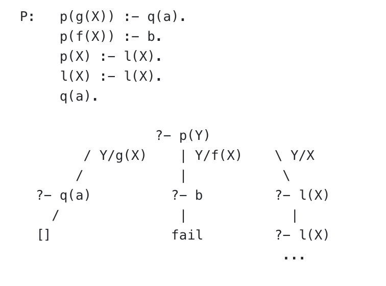
Resolution as a Tree search
Since clauses may have different resolutions, each resolution gets searched through backtracking, implying a tree structure. Indeed, the path from the main goal ?- C1 ... to ?- w(B1, ..., C2, ...) is an edge on the tree; each possible unifier\(w\) is a different branch from the root. The resolution of ?- w(B1, ..., C2, ...) is a subtree from \(w\)'s node.
Thus, a successful proof (a refutation) is represented by path from the root to an attempted resolution of an empty goal, which is a leaf. Note that leaves are either empty goals (successful resolution) or resolution failures, since these are the only cases that don't derive goals recursively.
A failure occurs when two expressions cannot be unified, e.g. they are non-variables with different values. When a failure is reached, the algorithm backtracks to the last successful resolution (i.e. the parent node) and evaluates the next unifier.
The set of root-{empty-goal} paths is the set of solutions to the query; prolog searches through this tree to find them. Since the resolution algorithm completes the first subgoal before moving on and backtracks on failure, the tree is searched using depth-first search.
Aside: BFS is not used because it takes up too much space
Aside: this seems to imply that although the order of clauses in the body of another clause doesn't affect the solutions of the program (i.e. is semantically equivalent), it will dictate the order that they are found.
Aside: once cuts are introduced, the order of the clauses does matter because cuts stop backtracking after a certain clause
Lecture 16 - Cut, Negation, and a Simple Interpreter
In Prolog, the cut! is a goal that succeeds when first reached, but fails if Prolog attempts to backtrack through it. So, it forces prolog to commit to the choices made before the cut.
?- q1, ..., qn,!, r1, ..., rn
Here, the first unification of q1, ..., qn is "locked in" by the cut, but backtracking is allowed in r1, ..., rn.
The cut is used to constrain the possible values returned by a predicate appearing earlier, e.g. if we only want to consider one unification of that clause. It is used to indicate clauses that don't need to be recalculated, often leading to performance improvements.
Aside: this behavior clearly can't be defined in terms of the syntax we've seen, so it must be doing something special, and is thus hard-coded into Prolog (i.e. is not surface syntax)
Aside: the cut can be characterized as a pruning of the resolution search tree; branches created by backtracking are "cut" off.
Note that since the cut prevents some of the resolution search from happening, the order of the goals (including the cut) now impacts that actual set of results returned.
Usage Example
In Assignment 3, my clique predicate was defined as
The cut is where it is so that we don't re-evaluate findall, since every permutation of the list of nodes is a valid unification to K. However, any order of K produces the same result, so checking all of them produces the same result as checking just one. So, the cut is added to prevent backtracking.
We can also use it to prevent "multiple matching" scenario when just one matching is sufficient, like for the function member.
% here, we have the cut so that we stop looking once we find the member% otherwise, the query would return n trues for n occurences of% X in the listmember(X, [X|T]) :-!.member(X, [H|T]) :- member(X,T).
Aside: having a cut as a first goal of a clause makes sure that it is only matched to once
Aside: having a cut as the last goal of a clause makes sure that the first "full" matching to the clause is the only one that occurs
Aside: this kinda characterizes the cut as an operator that can take "for all" problems (created by the universally quantified head) and turn them into "there exist" problems by stopping evaluation when one is found. Is it linked to the difference between the head and body of clauses, i.e. the quantifications?
Construction of Conditionals
We can use the cut to implement conditional logic. Here, we are expressing if p, then q, otherwise r.
x :- p,!, q.x :- r.
If p is unifiable (i.e. true), then we move onto unifying q; the cut prevents us from backtracking and finding r. If p is not unifiable (i.e. false), then we move onto the next clause r without ever checking q.
Aside: as alluded to in LISP, conditional logic has a special characterization that makes it different from a regular function: the fact that it can't evaluate all of its arguments (or it won't work). In Prolog, this is expressed through the special construct of the cut, which is analogous since it prevents evaluation. In fact, the direct equivalent of a cut in LISP would be some construct that prevented evaluation of a function, which is the conditional. So, the two are inexorably linked.
Negation
The negation operator \+ in prolog is equivalent to the logical not\(\lnot\).
It can be defined in terms of the cut:
not(X) :- X, !, fail.
not(X).
Aside: this follows the form of if-then-else: if X is true, then not(X) is false, else not(X) is true.
Aside: while programming in prolog, it can be useful to use negation to turn "for all" into "there exists". E.g. in the clique question, it is easer to check if a list is not a clique, since it comes down to if two nodes in the list don't share an edge, which can be checked with conjunctions, i.e. ,.
Semantics of Negation
The definition of negation in terms of cut implies that negation is the failure to prove, i.e. \+ P iff P is false, which seems to make sense. However, when variables are involved, this isn't always the case. For example, consider:
Here, we might expect ?- even(X) to produce 6., but it doesn't. odd(N) matches only weird, which isn't an integer, so the query fails.
This is because there is a slight difference between knowingeven(6) is true, and being unable to prove that odd(6) is false. Prolog is aware of this, and doesn't equate the two.
Prolog's Internal Database
Meta-predicates
Prolog has built-in predicates that directly affect the knowledge of the program (i.e. the database) at evaluation time, so they are useful for the DB.
Name
Description
assert(Clause)
Adds Clause to the current program being interpreted. Note that where in the program it gets added depends on implementation. E.g. assert(above(X, Y) :- on(X, Y)).
asserta(Clause)
Inserts Clause as the first clause for that predicate
assertz(Clause)
Inserts Clause as the last clause for that predicate
clause(Head, Body)
Searches the program for a clause whose head matches (i.e. unifies to) Head (i.e. searches for a clause). Head must not be a free variable.
retract(Clause)
The first clause matching Clause in the program is deleted
retractAll(Clause)
Every clause matching Clause in the program is deleted
Prolog as a Database
These meta-clauses enable us to use prolog like a simple database (which is quite fast), where predicates are used to encode attributes:
Insertion of a tuple: assert(pred(const)).
Deletion of a tuple: retract(pred(X)).
Query tuples: clause(Head, _).
A Prolog Interpreter in Prolog
We can write a prolog interpreter in prolog (homeomorphic spaces, iykyk).
% if we interpret true or the empty goal, the program must be trueinterp(true).interp([]).% interpreting a list of subgoals is like a conjunction, so we% defer to the conjunction in prolog (,)% tail-recursive case of interpreter% we have a cut so that the interpretation can only happen onceinterp([H|T]) :-!, interp(H), interp(T).% if there is a clause matching our program matching P, we evaluate that% this is the "search and match" step that prolog takes% the bindings for P's variables get passed to Y automaticallyinterp(P) :-clause(P:-Y), interp(Y).% next, we check if P is a built-in predicate by letting prolog evaluate it directlyinterp(P) :-P.% finally, if this fails, we can't evaluate the goal, so it fails and backtracks
Lecture 17 - Constraint Programming and Satisfaction
Constraint programming studies models of computation based on constraints, the main idea being that if a set of constraints can fully characterize a problem, finding a solution to the constraints solves the problem.
Constraint programming combines research from fields including AI, Programming Languages, Symbol Computing, and Computational Logic (!!!!!!!!)
Domains constraint programming have been applied to include graphics, NLP, DBs, Electrical engineering, etc (more examples in eclass writeup)
Examples of Constraint Problems
The following problems are (most?) efficiently solved using constraint programming.
Cryptarithmetic Puzzles
Cryptarithmetic puzzles are solved by assigning digits to letters (or more broadly, symbols); these symbols are related by an "equation" like the one below.
Since there are a finite number of digit-number pairings, a solution can always be guessed, but the test and guess approach is inefficient.
The "equation" is really a set of constraints, so a constraint logic program can solve it more efficiently
S E N D
+ M O R E
--------------
M O N E Y
N-Queens Problem
N-queens problem: If \(N\) queens are placed on an \(n\times n\) board, what is the smallest \(n\) such that a configuration exists where no two queens are in the same column or diagonal?
The search space for this problem is very large, but constraint programming can significantly reduce the amount of it that needs to be searched
NP-Complete Problems
These include the travelling salesman problem, map-colouring, planning problems, etc.
Constraint-Solving Approaches
When a problem is solved algorithmically, the programmer develops, implements, and runs an algorithm in a programming language; the work is coming up with this algorithm
When a problem is solved with constraint programming, the programmer must formulate/model the problem in the underlying language. The "algorithm" part is deferred to the language implementation
Aside: where does the line between programming language and AI lie? Simply describing a problem (albeit in a formal way) and having solutions generated seems like something additional to a programming language.
Aside: what we have been doing in prolog is, although expressed in an unfamiliar way, still algorithmic programming.
The two main constraint programming approaches are Boolean Satisfiability and Constraint Satisfaction, the latter of which we will study.
Constraint Satisfaction
Constraint Satisfaction Problem
Definition
A constraint satisfaction problem (CSP) consists of
A set of variables \(X=\set{x_1, \dots, x_n}\)
A domain\(D_i\), i.e. set of possible values, for each \(x_i\in X\)
These are often consecutive integers, but can be anything, including non-numbers
A set of constraints restricting which values variables can simultaneously have
A solution to a constraint satisfaction problem is an assignment of every variable to a value from its domain in a way where all constraints are satisfied.
E.g. for variables \(X, Y, Z\), with domains \(D_X, D_Y=\set{1, 2, 3}, D_Z=\set{2, 3, 4}\) and constraints \(X<Y, Y<Z\), the assignment set\(X=1, Y=2, Z=3\) is a solution
E.g. the eclass notes contain an expression of the N-queens problem
A single constraint is local (i.e. applies to just the variables involved), but a solution to all the constraints is global, (i.e. involves all the variables). So, a assignment set may satisfy a single constraint, but won't be a solution if it fails any others.
Systematic Search Algorithms
As alluded to, the generate-and-test paradigm (GT) that generates and test all possible value assignment sets is strictly correct, but inefficient.
The backtracking paradigm incrementally attempts to extend partial solutions towards complete ones by picking the "next" value in the domain for a variable. Backtracking occurs when a constraint-breaking value is picked.
Aside: this mirrors how prolog's resolution solver works
Aside: if an "earlier" variable doesn't affect some contiguous subset of the rest of the variables, work is still repeated. This suggests a DAG structure and corresponding algorithm could be used to improve the efficiency
Consistency Techniques
Constraints and the domains of their variables might make the set of constraints inconsistent, especially if some variables have already been bound.
Currently, we only discover an inconsistency when we try to assign variables, which is inefficient.
To improve, we will check for consistency initially and after each new assignment in order to discover values that aren't possible
Essentially, we are checking for values that are not possible to satisfy at our current place in the backtrack, implying we shouldn't search through them on this backtracking cycle.
A technique is applied to a constraint to reduce the domain of the variable(s) involved; a domain reduced to \(\emptyset\) indicates unsatisfiability.
Aside: the non-permanent removal of values from the search based on the current backtrack suggests a stack frame type structure (and therefore a recursive procedure) containing the current "context" (stack structure is also implied from backtracking)
Node Consistency
If a constraint has one unassigned variable (e.g. \(X>2\) or \(X = Y\) where \(Y\) is bound from previous backtracking), the variable's domain \(D\) can be filtered using the constraint as a predicate, i.e. all \(d\in D\) not satisfying the constraint are removed from \(D\)
I.e. all the direct constraints are used to prune the domain for a variable
A CSP where this process (ensuring node consistency) has been applied is node consistent
Arc Consistency
If a constraint has two unassigned variables \(X\) and \(Y\) and there is some value \(x\) for \(X\) where there is no value satisfying \(Y\) in its domain, this \(x\) can be removed the domain of \(X\) (for this backtrack).
E.g. for constraints \(X<Y, Y<Z\) from before, \(X=3\) cannot give a solution for \(Y\), so \(3\) is removed from the domain of \(X\), preventing further search. The arc-consistent version of this problem has domains \(\set{1}, \set{2}, \set{3}\) for \(X, Y, Z\) respectively.
A CSP where this process (ensuring arc consistency) has been applied is arc consistent
Aside: node consistency seems like a base case and arc consistency like an inductive case, implying that a complete satisfiability check can be done with these two techniques alone through an recursive structure
Constraint logic programming combines constraint programming and logic programming. In prolog, this can be achieved by embedding a constraint solver, which replaces prolog's unification process
Unification in prolog is a constraint solver, where the domains are equations (and thus, equations in prolog are related by conjunction, disjunction, negation, etc)
Aside: is it correct to say that Prolog is also a constraint solver over \(\mathbb{N}\) since it has support for equations over integers (and floating point numbers for that matter)?
Aside: how does differ from a boolean domain? The connectives seem to be the same
Constraint solvers are defined by their domains; common ones include finite domains (useful), \(\mathbb{R}\), \(\mathbb{Q}\), booleans, etc.
So, free variables are given a domain (e.g. \(\mathbb{R}\)), as opposed to regular prolog where they are simply uninstantiated. They can't be unified to anything anymore, so the whole program is constrained
Defining a global domain makes satisfiability problems possible and meaningful to solve; in prolog, the lack of such a domain makes free variables meaningless beyond being able to unify with anything
Aside: how are countably and uncountably infinite domains implemented? I assume some symbolic computation is necessary
Solving Strategy
A constraint programming language has a built-in set of primitive constraints, related to its domain. E.g. for domain \(\mathbb{R}\), this might include \(=\), \(<\), \(>\), etc.
All other constraints are representable in terms of the primitive constraints, whether they are defined this way or compiled into (possibly multiple) primitive constraints
Aside: turning user-defined constraints into primitive ones is an assembly step
Aside: this is directly analogous to the adequate connectives problem for boolean algebra; an adequate set of connectives is a valid set of primitive constraints because they can build anything. This implies a boolean algebra solver needs only the NAND primitive constraint
All the primitive constraints generated in the program are stored in the constraint store
The store is modified as the backtracking process adds and removes additional constraints to the program
Every time the store changes, we check for satisfiability, and backtrack if the program is not satisfiable
Example
% this program is defined over a number system, e.g. the naturals, reals, etcp(f(X)) :-X>1, q(X).q(X) :-X<5.% query?- p(Z).
Step
Program Evaluation
Constraint Store
1
?- p(Z)
{}
2
X > 1, q(X)
{Z = f(X)}
3
q(X)
{Z = f(X), X > 1}
4
X < 5
{Z = f(X), X > 1}
5
\(\varnothing\)
{Z = f(X), X > 1, X < 5}
Here, the constraint solver must then be used to determine if {Z = f(X), X > 1, X < 5} is satisfiable, which depends on the domain over which it is defined. These particular constraints are satisfiable over \(\mathbb{R}\), \(\mathbb{N}\), etc.
Constraints are defined where regular terms would be in prolog
Constraint Solving in Prolog
Both packages below (clpr and clpfd) come with SWI-prolog.
Solving over \(\mathbb{R}\)
The clpr (constraint logic programming over reals) library can be used in prolog to invoke a constraint solver over \(\mathbb{R}\)
:- use_module(library(clpr))
We program in prolog normally, but enclose constraints we want clpr to solve in curly braces {}
% here, we want X > 1 to be constraint-solved over the reals% q(X) should still be solved through unification, since it's a constraint on an equation, not a real numberp(f(X)) :-{X>1}, q(X).q(X) :-{X<5}.
Finite domains tend to be the most useful domains to solve constraints over because they are the best at representing "useful" problems, like scheduling, planning, packing, etc.
Structure of a clpfd Program
First, we must load the clpfd library
:- use_module(library(clpfd))
Specifying Constraints
The operators of constraints are prefixed with # to distinguish them from the regular prolog operators.
E.g. N #\= 0, A #> B
E.g. for the "SEND MORE MONEY" example:
% notice here how #= is used to define the constraint% but the regular * and + are used because they are regular arithmetic operationsS*1000+E*100+N*10+D+M*1000+O*100+R*10+E #=M*10000+O*1000+N*100+E*10+Y.
Both sides of the constraint can be arithmetic expressions, unlike regular prolog.
Restricting Domains
Note: the domains of variables can be constricted in regular prolog as well, e.g. in/2 and ins/2 restrict variables to being integers. We saw this done with things like number, atom, etc. as well
The in operator can restrict a value to a range, which is defined with the notation a..b corresponding to the range \([a, b]\). The union operator \/ can be used to join ranges.
X in 1..4% regular range[X, Y, Z] in 1..4% list of variables in rangeX in 1..4\/10..29% union of ranges
inf and sup can be used in ranges to represent \(-\infty\) and \(\infty\), respectively
Aside: are .. and \/ syntactic sugar or core language features?
The all_different/1 checks if a list of values are all distinct.
An example of the domain restrictions required for the SEND MONEY problem can be found on eclass.
Searching for Solutions
The labelling predicateslabel/1 and labelling/2 are used to tell the (clpfd) solver to solve the given list of variables, i.e. assign domain values to them in order and backtrack until a solution is found. This process is called labelling.
label([X, Y, Z]).
Sometimes, only a few variables need to be searched to assign labels because constraint propagation can solve the rest
Aside: since the order of the list is the order of evaluation, the order of the solutions depends on this list
Essentially, labelling is the process that turns constraints into lists of possible bindings for all the variables.
An implementation of label gives insight into how it works:
mylabel([]).% indomain matches if a variable V is in the global domain% backtracking through it leads to the domain values being matched in increasing order, mirroring the labelling structuremylabel([V|Vs]) :- indomain(V), mylabel(Vs).
Search Control Options
The labelling\2 predicate allows a list of search options/parameters to specify the orders of the variables and domains to be solved.
Variable order
Name
Predicate
Explanation
Leftmost
leftmost
The first variable is selected (default option)
Minimum
min
The variable with the smallest lower bound is selected
Maximum
max
The variable with the largest upper bound is selected
First-fail
ff
The variable with the smallest domain is selected (tiebreaking defers to leftmost)
Most constrained
ffc
Like ff, but tiebreaking defers to the largest number of constraints, then leftmost
Constraint order
Name
Predicate
Explanation
Upward
up
The constraints are considered in ascending order
Downward
down
The constraints are considered in descending order
Lecture 19, 20 - CLPFD Predicates and Reification
Local Constraints
Arithmetic Constraints
Arithmetic constraints are the same as their prolog counterparts, but prefixed with #: #=, #\=, #>, #<, #>=, #=<.
Boolean Operators
Name
Operator
Explanation
Logical Or
#\/
Logical or connective
Logical And
#/\
Logical and connective
Logical Not
#\
Logical not
Implication
#==>
The logical implication connective, equivalent to (#\ A) #\/ B. #<== also exists
Equivalence
#<==>
The logical equivalence connective ("if and only if"), equivalent to (A #==> B) #/\ (B #==> A)
These operators can turn true/false values into 1 and 0; this is an example of reification.
Aside: the symbols representing or#\/ and and#/\ directly relate to the union \(\cup\) and intersection \(\cap\); in prolog, these are directly expressed unions and intersections when they relate domains (sets), instead of predicates. This equivalence can happen because both "things" are instances of boolean algebras
Global Constraints
Global constraint predicates have built-in constraint prorogation; they affect the whole program instead of just the expressions they relate. Generally, their clpfd implementations are more efficient than their user-defined ones.
Aside: this implies that something other than just node/arc consistency is going on
Predicates
alldistinct\1: checks if a list of domain variables has no duplicate values
sum(+L, +relOp, value) checks if the sum of list L is relOp (e.g. =, \=, >, etc.) the value
Aside: note that because prolog has the "'return value' as parameter" structure, the equality check must be defined in the predicate instead of being an operator on its own and getting parsed into the AST
Aside: all the prolog predicates we've seen have implicitly had = as a relational operator, but here we are specifying it. Why hasn't this been a thing before? We have had more relational operators…
Aside: this moves the relational operator from the body as a clause relating the variables in the predicate to an argument of the predicate itself
Aside: The nested expressions → prolog conversion is reverse polish notation; expressions nested with () get "compiled" out into the body of a prolog clause as conjunctions, flattening them
Reification
Reification is the process of turning a constraint into a variable (in clfpd) that holds the value true or false. So, we can explicitly reason about whether the variable (and thus the constraint) is true or not within the program itself.
The operators defined in the next section (i.e. the ones prefixed with #) are used to reify the constraints
Since prolog doesn't have (and is designed in a way that doesn't need) boolean values, booleans are represented by 0 and 1
Aside: This explicit reasoning about true/false values in the context of constraints is different than our predicate-built approach before; this is why things like logical connectives can be defined and used instead of just predicates: we are reasoning with true and false values directly now.
Aside: all clfpd does is add a domain. What about adding a domain to prolog makes it possible to have non-built-in logical connectives now?
Aside: this idea needs more consideration
In natural language (english), reification is the process of making something abstract more concrete, sometimes by replacing an abstract concept with a particular instance.
So, "reify" is an antonym to "abstract" or "generalize"
Reification Example - occurs
% NOT REIFIED% queryq(I,L,N) :- length(L,4),L ins 1..10, occur0(I,L,N), label(L).% predicate: occur0% defined occur0(_,[],0).occur0(I,[I|L],N) :-N#=N1+1, occur0(I,L,N1).occur0(I,[J|L],N) :-I #\= J, occur0(I,L,N).% REIFIED% queryt(I,L,N) :- length(L,4),L ins 1..10, occur(I,L,N), label(L).% predicate: occuroccur(I,Vars,N) :- generate_list(I,Vars,L), sum(L,#=,N).% helper function: generate_list (encapsulates occur0 logic, written in a reified way). The generated list is an indicator vector; entries 0 mark "don't occur" and 1 the oppositegenerate_list(_,[],[]).% we define the check in terms of boolean logic directlygenerate_list(I,[A|R],[T|S]) :- (I #= A #==> T#=1), (I #\= A #==> T#=0), generate_list(I,R,S).
Appendix: General Answer Set Programming Interpretation of Reification
Shoutout to Spencer for explaining this on the discord and providing the example
In ASP in general, reification turns a "regular" program (e.g. a prolog program) and turns it into something that another program can reason about; this "other program" may be a constraint solver, for example.
Transforming constraints → boolean values happens because (mostly) any program can reason in terms of boolean values
Aside: this example of reification seems analogous to the assembly (or maybe even compilation step in the execution of an imperative program); the program is transformed into a form that the underlying interpreter (?) can use
An example of reification is below:
% non-reifiedbagel(1,2,3). bread(42) :- bagel(1,2,3).% reified% aside: what is this representation and how is the reification step implemented?atom_tuple(0). atom_tuple(0,1). literal_tuple(0). rule(disjunction(0),normal(0)). atom_tuple(1). atom_tuple(1,2). rule(disjunction(1),normal(0)). output(bagel(1,2,3),0). output(bread(42),0).
Lecture 21 - Answer Set Programming
Answer set programming is a declarative programming paradigm for problem/constraint solving and knowledge representation.
Problems are defined in terms of the rules that govern their actual set of solutions. Stable models or answer sets are solutions to a problem
Programs
We encode problem instance\(Q\) in a program \(P\), expressed as non-monotonic logic. Stable models of \(P\) are computed by an ASP solver; these correspond to the solutions to \(Q\).
This encoding should be "bijective": each solution should have a stable model, and if no solutions exist, there are no stable models
A normal program is a finite set of rules of the form \(A \leftarrow B_1 \dots B_k, \text{ not } C_1, \dots, \text{ not } C_n\), read "If \(B_1\dots B_k\) are in a solution but none of the \(C_i\) are, then\(A\) is in the same solution". The terms \(A, B_i, C_i\) are atoms in the underlying propositional language.
This is the most basic form of program
\(\text{not}\) is default negation
Aside: how does this differ from other types of negation.
\(A_i\), \(\text{not } C_i\) are literals
Aside: because the atoms are defined in an underlying propositional language, this reasoning can be applied to any propositional language
Aside: formally, what is a propositional language?
Aside: is \(\leftarrow\) semantically different than :-?
Programs can be written with variables to generalize non-ground rules over all the constants in a program. Like in prolog, variables are denoted with capital letters.
A constraint is characterized by a rule with an empty (false) head; semantically, this rule cannot apply to any instance, so can't exist in the program at all.
Grounding
A ground program is a program that doesn't contain any variables and has the same answer set as some original program. Grounding is the process of translating a non-ground program into a ground program.
If a non-ground program has a finite number of constants and no function symbols, grounding it leads to a ground program
Function symbols represent functions that are outside of the domain that the ASP solver has to deal with. So, we almost treat function symbols as symbols that can exist structurally (i.e. hold variables), but don't hold semantic meaning to the ASP solver (and thus are not evaluated).
Aside: we could also abstract function symbols away as things that can be evaluated into expressions of variables and values that we can reason about
More examples are in the [[intro-ASP-for-c325 (1).pdf|class slides]].
Answer Sets
Answer Set
Definition
An answer set or stable model\(M\) of program \(P\) is a subset of the rules of grounded \(P\) that satisfies the following properties
\(M\)satisfies every rule in \(P\)
For any rule\(A \leftarrow B_1 \dots B_k, \text{ not } C_1, \dots, \text{ not } C_n\), \(a\in M\) if all \(B_i\) are in \(M\) and no \(C_i\) are in \(M\), then the rule \(A\in M\)
For any "answer" \(h\in M\), there is a corresponding rule \(h \leftarrow B_1 \dots B_k, \text{ not } C_1, \dots, \text{ not } C_n\), \(a\in M\) if all \(B_i\) in the program where all \(B_i\) are in \(M\) and no \(C_i\) are not in \(M\)
We say \(h\) is supported by the rule
Any atom in an answer set must be justified, i.e. supported by a non-circular derivation
Aside: the process of finding an answer set is like "shrinking down" the the rules of the program to a point where its meaning is defined as a list of constants; these shrunk subsets model the program.
Essentially, an answer set is a set of attributes on the constants of a program that satisfy all of the rules and facts of \(P\). A program may have many, one, or no answer sets.
Finding Answer Sets
First, the program is grounded replacing all the variables with variable-free terms and (presumably) instantiating all the general rules with the appropriate constants to turn them into facts.
Aside: this is analogous to an assembly step.
LParse is a program that can perform this step for programs written in its standard syntax
Then, an ASP solver is called that turns the rules into a set of models that satisfy it.
Aside: this is analogous to an evaluation step.
ASP Language Features (Lparse)
Sets are denoted with \(\set{a_1; \dots; a_n}\) (i.e. with \(;\) delimiters), or \(\set{a_1, \dots, a_n}\) in earlier LParse syntax.
A cardinality constraint\(x \set{a_1, \dots, a_n} \, y\) for \(x, y\in \mathbb{N}\) specifies any subset of \(\set{a_1, \dots, a_n}\) with size between \(x\) and \(y\) inclusive, i.e. \(x \leq \#\set{a_1, \dots, a_n} \leq y\).
Cardinality constraints of the form \(0 \set{a_1, \dots, a_n} \, n\) are called choice constraints and are satisfied by any subset of \(\set{a_1, \dots, a_n}\)
Sets can be expressed concisely using the conditional literal\(a : D\), where \(a\) is an atom and \(D\) is a domain predicate. Roughly, it specifies the set of atoms \(a\) that satisfy the domain predicate \(D\).
E.g. \(1 \set{\text{setColor}(v,C): \text{color}(C)}1\) is shorthand for \(1\set{\text{setColor}(v,\text{red}); \text{setColor}(v,\text{blue}); \text{setColor}(v,\text{yellow})} 1\)
ASP vs. Prolog
ASP an Prolog have similar syntax (ASP isn't strictly a language, but the syntax of LParse is a common standard), but different paradigms.
In Prolog, we define a knowledge base in terms of rules and facts, then run queries over it; computation happens when "evaluating" these queries by resolution.
In ASP, we still define knowledge and rules, but the program has a solution that it evaluates to, namely the list of answer sets. ASP is a more faithful adaption of horn clause logic than prolog.
There are cases where prolog doesn't terminate, but the equivalent ASP program does (aside: what kind of cases?)
Lecture 22 - Answer Set Planning
Planning is a problem in AI that concerns autonomously finding a sequence of steps (a strategy) to solve a given problem.
For a fixed number of steps, this problem is NP-complete.
Representing Planning Problems
In a planning problem, we need to represent the following:
Steps in a plan.
Note: we are representing time passing by adding a "timestep" argument in a predicate and implementing the constraints of time (e.g. it moves forward, etc) manually.
time(0..steps) % steps are integers that start at 0next-state(T2,T1) :-T2=T1+1% integers increment by 1
Fluency: properties that are held constant across time by default, unless they are changed by an action.
Here, we define facts with a variable representing time, i.e. matching any time.
These rules are called fluents.
on(a, table,T) % objects stay on tables by default.
Actions: things that happen at a given time step that change the state of the world
The solution generated is a chronological series of actions
move-to(a, b,T) % object a is moved to place by
The initial state of the world
We define facts where the timestep is \(0\).
on(a, b,0).on(b, table,0).
The goal state of the world
A rule with time as a "parameter" specifying what we want to occur
% we define what the goal isgoal (T) :- time(T), on(a,c,T), ...% we state that the goal must be satisfiedgoal :- time(T), goal(T).:- not goal.% not solving the goal is a constraint.
Actions
To generate the sequence of actions that is our solution, we need to know
Which actions should be chosen under which conditions
Which objects are affected by the action
Any effects the actions have on objects
This is analogous to a side-effect; the state of the program changes. Note that the state of the program is the product-type containing the states of the objects
We also must assume the frame axiom: if an object isn't affected by an action at a given state, then the fluents must preserve the current state of the object.
The following scheme represents an action system in ASP:
% an action may have pre-conditions that must be metaction(Obj,T) :- pre-conditions.% **conflicting actions** can be defined by the constraint that both cannot happen at the same time.% if not specified, then any actions can happen at the same time.:- action(Obj,T), conflicting-action(Obj,T).% we can define if an action affects an objectaffected(Obj,T) :- action(Obj,T).% an action changes the property of an object % this is esentially an action definitionproperty2(Obj,T+1) :- action(T), property1(Obj,T).% fluencyproperty(Obj,T+1) :- not affected(Obj,T), property(Obj,T)
Note that we can define that only one action can happen per time step by defining the following conflict constraint
:- action(Obj1,T), action(Obj2,T).
We can define auxiliary predicates to tell us information about the state; these are not used to find the actual solution.
Aside: Planing Problems as Graphs
We can represent planning problems as a graph.
The different states of the world are nodes
Actions are edges connecting the notes, since they change the state.
This also illustrates which actions can't be taken (no edge), which states are unreachable (components of the graph), etc.
We start at the node representing the initial state; we try to move along edges to reach the node representing the goal state.
Problem can be solved: path exists both states
This lets us use graph-theoretical knowledge and algorithms to solve planing problems.
This interpretation follows from the fact that predicates over a set are inherently a graph structure.
Lecture 23 - Foundations of Logic Programming
[[logic-foundations-w2024.pdf|Notes]]
1. Syntax of Logic Systems
The syntax of a logical system defines which logical expressions, constructed from logical symbols are legal, i.e. well-formed.
A given logical syntax contains an alphabet, i.e. a lexicon of the symbols that may be used. These usually include:
Constants
Functions: defined in some other system the logical system cannot interact with, like arithmetic over \(\mathbb{N}\). We are only concerned with the fact that a symbol representing a function exists; not its actual definition.
Predicates: defined as subsets of \(A\times B \times C \times \dots\), where \(A, B, C, \dots\) are the arguments of the predicate.
Variables: can represent any constant in the domain, get constrained.
Connectives: operators that operate on and produce truth values.
Quantifiers: operators that operate on members of the domain to produce truth values.
Punctuation: specify the precise meaning of expressions and make them more readable, e.g. (, ), ,, etc. This can also include text like "such that", "where", etc.
2. Semantics of Logic Systems
The semantics of logic defines the relationships between formulae.
For set of formulae \(\Sigma\) (interpreted as the conjunction \(\displaystyle\bigwedge\limits_{i=1}^{|\Sigma|}\Sigma_i\)) and formula \(A\), we define the relation\(\Sigma \vDash A\) to mean that every way of interpreting (evaluating) \(\Sigma\) that makes it true also makes \(A\) true.
We say \(\Sigma\) implies \(A\), \(A\) follows from \(\Sigma\), \(A\) is a theorem of \(\Sigma\), \(A\) follows from \(\Sigma\), etc.
For propositional logic, since there are a finite number of possible assignments over propositions (since there are a finite number of variables), we can simply define logical consequence by constructing a truth table, i.e. testing every possible value.
However, this is infeasible in practice: propositions over \(N\) variables have \(2^N\) possible valuations.
3. Inference Rules of Logical Systems
For predicate logic, since we have quantifiers, there may be an infinite number of valuations for a given formula, so we can't simply use a truth table.
Instead, we use an inference system, which consists of a collection of inference rules that can be used to derive new formulae from existing ones.
Inference systems must be sound: new formulae must be logical consequences of the existing ones.
Inference systems may be complete (every logical consequence can be derived), but it is not strictly required, although it is nice to have.
Resolution is the inference system behind prolog; it is useful for this because it can be performed mechanically. But more elegant and human-meaningful ones exist.
4. Predicate Logic
Our main question is what the logical consequences of a horn clause L1 <- L2, ..., Lm is, where the variables are all universally quantified (\(\forall\)).
First, we consider the logical consequences on atoms without variables (ground terms).
We define the Herbrand Universe\(H_u\) as the set of all "objects" we can use predicates to relate (ground terms); specifically:
Any constant \(C\in H_u\)
If \(f\) is a function with arity \(n\) and \(t_1, \dots, t_n\in H_u\), then \(f(t_1, \dots, t_n)\in H_u\) as well
This function is (presumably) defined outside the logical system, so their actual definition doesn't matter; all that matters to us is that a function symbol exists
Nothing else is in \(H_u\)
We define a ground atom as any atom whose variables are instantiated by terms in \(H_u\). We can construct the set of ground atoms that are logical consequences of \(P\) iteratively:
We start with the empty set \(S_0\)
\(S_1\) contains any \(H\) from \(P\) where H :- B1, ..., Bn where \(B_1 \dots B_n\) are constants in the program.
In general, \(S_{n+1}\) contains everything in \(S_n\), as well as every instance of a clause \(H\in P\) where H :- B1, \dots, Bn and \(B_1 \dots B_n \in S_n\)
This process stops if \(S_n = S_{n+1}\) for some \(n\)
By definition of this process, everything in a given \(S_i\) is a logical consequence of \(P\).
Note: This process may never stop; there may be (and often is) an infinite number of logical consequences of \(P\).
The remaining material is optional
Lattices and Fixed point Theorem
The Knaster-Tarski fixed-point theorem states that every monotonic operator defined on a complete lattice has a fixed point that can be computed iteratively by repeatedly applying the operator on the "first" element of the domain.
I.e. a member of the domain \(S\) exists such that \(T(S)=S\) for operator \(T\)
A lattice is a partial order; completeness implies the existence of a GLB and LUB exist
This sequence of computational steps can be characterized as the repeated application of an operator to a set, namely \(S_0\). We define this operator as \(T_P(S) = \set{a \mid a \leftarrow b_1, \dots, b_n \text{ is a ground instance of a clause in } P, b_1 \dots, b_n \in S}\). We can show that the fixed-point theorem applies:
Monotone: in our case, this means \(S_1 \subseteq S_2 \implies T_P(S_1) \subseteq T_P(S_2)\), which is trivial
The least fixed point of is the set of ground atoms that are logical consequences of \(P\).
Introduction
I had fun with this course; it should be obvious from all the asides. Hope they are well received :)
Appendix 01 - Accumulators
An accumulator is a parameter that is used to accumulate the result of a function, usually by passing (cons x Acc) into the recursive call
Often used with a helper function that calls the accumulator version of the function with an empty list for the accumulator
We install SWI-prolog and start it by typing swipl into the terminal. This opens a session. Prolog can be used exclusively from the terminal, where each line adds to the program.
To load a program from a file (which is how any development will happen), we type
[fileName].
Here, we do not use the file extension
Aside: as far as I know, this just appends everything in the file to the "session"
If the program is valid, it will return true and print that to the terminal. Otherwise, it will print false. It may also provide warnings about your program; most commonly, that you have a singleton variable that should be a _ instead.
Queries
Prolog programs define knowledge, and "execution/evaluation" happens by running a query over the program's knowledge. Prolog prompts you for queries with ?- in the terminal, once a program has been loaded.
Like anything else, queries end with ..
When a query evaluates, it prints the result. If there are more results (i.e. the query can be unified more than one way, we can press ; to move through all the results). Once the last result has been reached, the query will "finish" and prolog will prompt you for another query with ?-.
Aside: ; is prolog's or; this ties into the fact that a query returning multiple results is a type of disjunction (i.e. this result or that result)
Debug
Ports
Regular prolog has four ports that describe the steps taken in program evaluation: Call for predicates getting evaluated, Exit when a clause is done being evaluated, Fail when a predicate cannot be unified, and Redo when a previously evaluated predicate is evaluated with different bindings after a backtrack.
SWI-prolog also has a Unify port, indicating unification of a clause.
Tracing
We can trace how a program evaluates through all of the ports.
?- trace, predicate(arg1, arg2, etc...)
This will show us the port used at each step, and prompt us with what to do next. Use creep to move to the next step.
The visibility of each port in the trace can be controlled, which is useful. For example, we might only care about where the program fails, so we wouldn't look at the Call port
?- visible(+port)# make port visible?- visible(-port)# make port invisible
leash and spy can further be used to control which ports are visible.
Exit
Prolog can be exited by pressing e (for exit) in the terminal (^D also kills the process, but is less graceful).
If a query (or rather, its process) is currently evaluating, it can be stopped by entering a (for abort); this will give you debug information and prompt you with another query. This is useful if your program has an infinite loop; you can get out of it without restarting prolog entirely.
Other
Prolog will guess if you make typos; these are most commonly capitalization errors, but actual mistypes are also detected. Typos are only detected if they are "close" to an exiting predicate or variable by one of the errors above. If a typo is detected, it won't execute the program until you either correct it or confirm you want to run the query you entered.
If we want prolog to fail an undefined predicate (instead of raising an exception), we can declare ?- dynamic(predicateName) before we run the rest of the queries. We can also include this in the program, but it is most useful for debugging.
Appendix 03 - My Final Exam Cheat Sheet
A common problem with making cheat sheets in an instinct to provide as full as summary of the course as possible. In theory, this maximizes its usefulness for an arbitrary student, but not necessarily for any particular student. Being aware of this, I created this cheat sheet with my own weaknesses in mind; its weighting of concepts does not represent that of the course. In particular, it favours logic programming concepts, since those were less familiar to me at the time.
E.g. (a . nil) is the same (a)
Simplest form: Representation with the least amount of dots. To get it: Dots . followed by open parentheses( and the matching closed one.
Alpha (\(\alpha\)) reduction: renaming a variable that is already bound, Beta (\(\beta\)) reduction: given an expression, replace all occurrences of parameters with the argument specified. Use alpha when beta fails due to a naming conflict. A lambda expression that cannot be further reduced by beta reduction is in normal form
Normal Order Reduction (NOR): evaluate the leftmost outermost function application f(g(2)) -> g(2) + g(2) -> 3 + g(2) -> 3 + 3 -> 6. Applicative Order Reduction (AOR): evaluate the leftmost innermost function application f(g(2)) -> f(3) -> 3 + 3 -> 6.
Church Rosser: If A → B and A→C reductions exist, then a D exists where B → D and C → D. Pt 2. If A has normal form E, then there is a normal order reduction A → E. If a normal form exists, NOR guarantees termination.
ADD = (λwzsx | ws(zsx)), T = (λxy | x), F = (λxy | y), IF = (λxyz | xyz), NOT = (λx | xFT), AND = (λxy | xyF), OR = (λxy | xTy), Y = (λy | (λx|y(xx)) (λx|y(xx)))
A closure is a pair \([\lambda, \text{CT}]\), where \(\lambda\) is a lambda function and \(\text{CT}\) is a (possibly empty) context, Always \(\cup \text{CT}_0\). Lambda functions: evaluate to a closure which contains the function body, variable list, and the context when the function was defined. Parts of a closureC: params(C), body(C), names(C), values(C)
The evaluation stack is used to evaluate expressions, The environment is used to keep track of bindings, The control is used to store instructions, The dump is used to store suspended invocation context, i.e. eval that we will come back to later
Built-in functions: A built-in LISP function (OP e1 ... e2) is compiled to "SECD language" instructions (ek' || ... || e' || (OP)) , If-then-else: the LISP function (if e1 e2 e3) is compiled to e1' || (SEL) || (e2' || (JOIN)) || (e3' || (JOIN)), E.g. (* (+ 6 2) 3) is compiled to (LDC 3 LDC 2 LDC 6 + *), || is append, (* (+ 1 2) (- 3 4)) becomes RP-notated 4 3 - 2 1 + *, Lambda Functions: A LISP lambda function (lambda (arg1 ...) (body...)) is compiled to (LDF) || (body' || (RTN)), Function application: A LISP function application (e e1 ... ek) is compiled to (NIL) || ek' || (CONS) || ... || (CONS) || e1' || (CONS) || e' || (AP), Scoping (let) statement: A LISP let statement (let (x1 ... xk) (e1 ... ek) exp) is compiled to (NIL) || ek' || (CONS) || ... || e1' || (CONS LDF) || (e' || (RTN)) || (AP), (letrec (f1 ... fk) (e1 ... ek) exp) is compiled to (DUM NIL) || ek' || (CONS) || ... || e1' || (CONS LDF) || (exp' || (RTN)) || (RAP), E.g. ((lambda (z) ((lambda (x y) (+ (- x y) z)) 3 5)) 6) compiles to (LD (1.1)), (LD (1.2)), (LD (2.1))
For goal ?- C1, C2, ..., Ck, we evaluate each subgoal from left to right, We evaluate by finding a clause in the program whose head "matches" the subgoal, replacing the subgoal with the body of the clause (applying variable bindings if necessary), and (recursively) evaluating that. If the subgoals are eventually solved, the original goal is as well
However, some unifiers are more general than others; \(w_1\) is more general than \(w_2\) if \(w_1\) can be obtained from \(w_2\) (by variable replacement), but \(w_2\) cannot be obtained from \(w_1\). Any unifiable \(t_1\), \(t_2\) have a uniquemost general unifier.
is arithmetic matching, = unifiable, =:= value of arithmetic expressions are equal, =/= not equal value of arithmetic, == syntactically equivalent. findall(X, Q, L) Binds to list L a list of all values for X that satisfies query Q, e.g. findall(X, likes(X, Y), L). X should parametrizeQ
clause A :- B1, ..., Bn, goal ?- C1, ..., Ck, We first proceed by attempting to unify the first goal C1 with clause A. If unifier\(w\) unifies C1 and A, the new goal, called a derived goal, becomes: ?- w(B1, ..., Bn, C2, ..., Ck). If the new goal is empty we have found a unifier.
cut! is a goal that succeeds when first reached, but fails if Prolog attempts to backtrack through it. So, it forces prolog to commit to the choices made before the cut. having a cut as a last goal in the clause makes sure only one solution gets returned.
% here, we have the cut so that we stop looking once we find the member
% otherwise, the query would return n trues for n occurences of
% X in the list
member(X, [X|T]) :- !.
member(X, [H|T]) :- member(X, T).
if p, then q, otherwise r: x :- p, !, q. x :- r.not(X) :- X, !, fail. not(X).(this defines negation+). Negation means definitely false, not unable to prove. So even(N) :- \+ odd(N), integer(N). integer(6). odd(weird). ?- even(X) fails
Insertion of a tuple: assert(pred(const)).Deletion of a tuple: retract(pred(X)).Query tuples: clause(Head, _). assert(Clause) (assert(above(X, Y) :- on(X, Y))), asserta(Clause), assertz(Clause), clause(Head, Body), retract(Clause), retractAll(Clause)
A constraint satisfaction problem has a set of variables, a domain those variables are in, and a set of constraints over the variables. The constraints can be "assembled" into primitive constraints and put in the constraint store. A solution is a set of bindings for the variables that satisfy all the constraints.
Node consistency: constraints like \(X>2\) are checked an values not satisfying them are removed from the domain. Arc consistency: constraints defined in terms of one variable that remove some from the others domain. E.g. \(X<Y, Y<Z\) from before, \(X=3\) cannot give a solution for \(Y\), so \(3\) is removed from the domain of \(X\), preventing further search. Consistency is checked at every step of. asearch to prune it.
X in 1..4, [X, Y, Z] in 1..4, X in 1..4\/10..29, all_different/1, label([X, Y, Z]).label/1 and labelling/2 are used to tell the (clpfd) solver to solve the given list of variables, i.e. assign domain values to them in order and backtrack until a solution is found. Impl: mylabel([]). mylabel([V|Vs]) :- indomain(V), mylabel(Vs).
Or #\/, AND #/\, NOT #\, implication #==>These operators can turn true/false values into 1 and 0; this is an example of reification.
We encode problem instance\(Q\) in a program \(P\), expressed as non-monotonic logic. Stable models of \(P\) are computed by an ASP solver; these correspond to the solutions to \(Q\). A normal program is a finite set of rules of the form \(A \leftarrow B_1 \dots B_k, \text{ not } C_1, \dots, \text{ not } C_n\), read "If \(B_1\dots B_k\) are in a solution but none of the \(C_i\) are, then\(A\) is in the same solution". The terms \(A, B_i, C_i\) are atoms in the underlying propositional language. A constraint is characterized by a rule with an empty (false) head. A ground program is a program that doesn't contain any variables and has the same answer set as some original program. Grounding is the process of translating a non-ground program into a ground program.
A cardinality constraint\(x \set{a_1, \dots, a_n} \, y\) for \(x, y\in \mathbb{N}\) specifies any subset of \(\set{a_1, \dots, a_n}\) with size between \(x\) and \(y\) inclusive, i.e. \(x \leq \#\set{a_1, \dots, a_n} \leq y\). Conditional literal \(1 \set{\text{setColor}(v,C): \text{color}(C)}1\) is shorthand for \(1\set{\text{setColor}(v,\text{red}); \text{setColor}(v,\text{blue}); \text{setColor}(v,\text{yellow})} 1\)
Planning problems: steps: time(0..steps), next-state(T2, T1) :- T2 = T1+1, fluency: on(a, table, T), actions: move-to(a, b, T), initial state on(a, b, 0). goal: goal (T) :- time(T), on(a,c,T), ..., goal :- time(T), goal(T). :- not goal. the frame axiom: if an object isn't affected by an action at a given state, then the fluents must preserve the current state of the object.
Sound: new formulae must be consequences of existing ones. This is required, completeness is not. We define the Herbrand Universe\(H_u\) as the set of all "objects" we can use predicates to relate (ground terms); specifically: An any constant \(C\in H_u\), If \(f\) is a function with arity \(n\) and \(t_1, \dots, t_n\in H_u\), then \(f(t_1, \dots, t_n)\in H_u\) as well. We define a ground atom as any atom whose variables are instantiated by terms in \(H_u\). In general, \(S_{n+1}\) contains everything in \(S_n\), as well as every instance of a clause \(H\in P\) where H :- B1, \dots, Bn and \(B_1 \dots B_n \in S_n\) (\(S_0\) is the empty set)