MATH2??Multivariable calculus is a superset of single variable calculus; it is the more general form of single-variable calculus.
In single-variable calculus, every object (point, value of function at point, derivative, second derivative, integral, etc) is a scalar. In multivariable calculus, this is not true: some of these objects remain scalars, become vectors, become matrices. Seeing what becomes what deepens one's understanding of single-variable calculus.
A multivariable function is defined as \[f(x_1, x_2, \dots, x_m) := (f_1(x_1, \dots, x_m), f_2(x_1, \dots, x_m), \dots, f_n(x_1, \dots, x_m))\]
Reasoning about multiple values as inputs and outputs doesn't fit well with the existing calculus we know. We can construct multivariable functions from single-variable functions (e.g. using Currying).
It is equivalent to think of a function of multiple variables as a function mapping vectors to vectors. The equivalent function looks like \[f(\vec{x})=\displaystyle \begin{bmatrix} f_1(\vec{x}) \\ f_2(\vec{x}) \\ \vdots \\ f_n(\vec{x}) \end{bmatrix}\]
for \(\vec{x}\in \mathbb{R}^{m}\) and \(f_?(\vec{x})\in \mathbb{R}^n\).
It also makes more sense to thing of multivariable functions to attach values to points in some high-dimensional space. For example, functions \(f: \mathbb{R}^{2} \to \mathbb{R}\) assign a scalar value to every point in 2D Euclidean space.
With all the output slots depending on all the inputs slots, there's just so much more going on here. Adding a new dimension is \(O(n^2)\) in a sense that we don't see when doing calculus to single variable functions. We will need linear algebra to handle this additional complexity.
Note: implicit functions of \(x\) and \(y\) (e.g. \(x^2+y^2=r^2\)) can be seen as explicit functions mapping points in \(\mathbb{R}^2\) to some constant by using subtraction to move all the \(x\) and \(y\) terms to the left of the equation.
The following can be assigned to a "dimension"
Magnitude of vector (\(\ell_2\) norm): \(\| (a,b) \|=\sqrt{a^{2}+b^{2}}\)
Dot product (inner product): \(\vec{a}\cdot \vec{b}= \| \vec{a} \| \| \vec{b} \| \cos(\theta) = \displaystyle\sum\limits_{n=0}^{\infty} a_n b_n\)
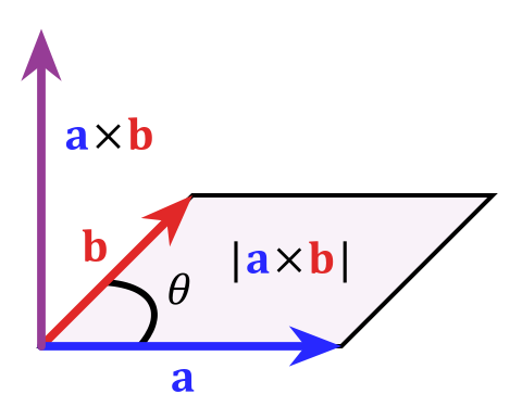
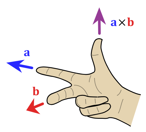
Cross product (\(\mathbb{R}^3\)): \(\vec{a}\times \vec{b}\) is vector \(\vec{c}\) such that \(\vec{a}\cdot \vec{c}\), \(\vec{b}\cdot \vec{c}\) \(=0\), i.e. \(\vec{c}\) is orthogonal to both \(\vec{a}\) and \(\vec{b}\).
Vectors are just matrices where one of the dimensions is \(1\). This implies a difference between column vectors and row vectors.
Matrix multiplication: the value of an entry is the dot product of the corresponding row of the first matrix and the corresponding column of the second matrix
The columns of a matrix are the new positions of the standard basis vectors. So, \(\begin{bmatrix} 1 & 1 \\ 0 & 1 \end{bmatrix}\) maps \(\begin{bmatrix} 1\\0 \end{bmatrix}\) to \(\begin{bmatrix} 1\\0 \end{bmatrix}\) (i.e. leaves it unchanged) and maps \(\begin{bmatrix} 0\\1 \end{bmatrix}\) to \(\begin{bmatrix} 1\\1 \end{bmatrix}\).
The determinant is a scaling factor. If the determinant is \(0\), the entire space gets squeezed down at least a dimension, and so the transformation is not invertible.
Hand-wavy determinant definition of the cross product: 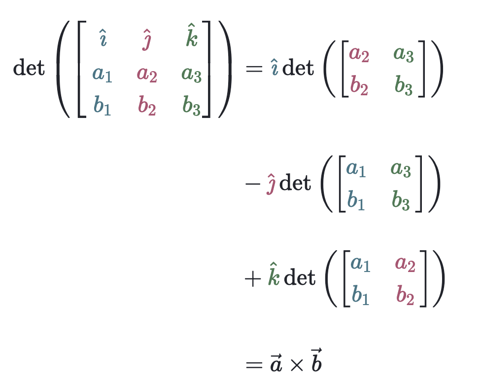
We can take "slices" of a graph by considering the intersection of the graph's surface with a plane. If that plane coincides with a standard basis vector in the input space, we end up simply looking at variation in one input element while keeping the rest constant. This "looks like" (is isomorphic to) a one-dimensional function.
We can understand the nature of a complicated surface by considering its slices as the "constant" elements are varied.
If we consider the intersection of many equally spaced horizontal planes with our functions, we get a nested set of slices called contours/isolines. These help us visualize the height of \(\mathbb{R}^{2}\to \mathbb{R}\) functions without needing to project them into the full \(3\) dimensions. Contour maps are used on maps of hilly terrain (e.g. mountains) for this reason.
Parametric functions describe curves using a parameter \(t\) that iterates over a fixed interval. So, parametric functions are of the form \(f : [a_1,b_1]\times\dots\times [a_m,b_m] \to \mathbb{R}^n\), usually for \(n\geq 2\).
The "dimension" of the parametric function's output is defined by the number of input variables. The space in which this output exists is defined by the number of output variables.
We parametrize a line/surface/etc by defining a parametric function that describes it. This maps every point in the input space to a point on the parametric object, which is useful for defining "coordinate systems" on arbitrary shapes.
Note: we loose a dimension of information when drawing a parametric plot, since we don't know what specific input values correspond to points in the output. We can add a dimension of visualization (e.g. color, transformation, etc) to illustrate this.
For \(\mathbb{R}^{2}\to \mathbb{R}^{2}\) functions, we can draw arrows to communicate direction and color (or length) to indicate magnitude:
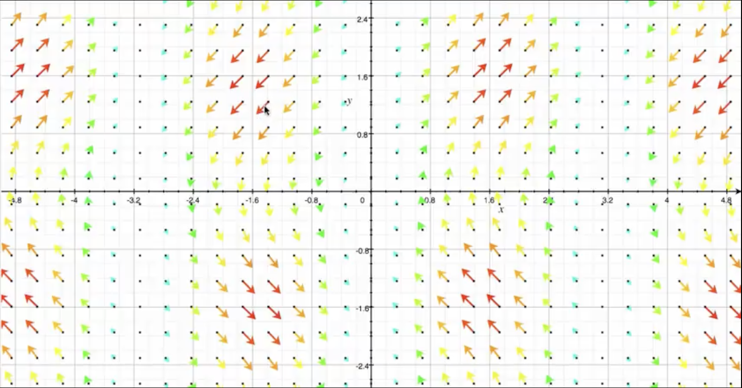
We can also visualize vector fields by imagining/animating how a fluid would flow around the input space if it "followed" the output vectors.
We can visualize \(\mathbb{R}^{3}\to \mathbb{R}^{3}\) functions with a corresponding 3D render.
We can visualize transformations by illustrating the "blank" input space (e.g. as a set of axes with gridlines), then moving each point in that space to its corresponding place in the output space.
\(\mathbb{R}\to \mathbb{R}\) transformation
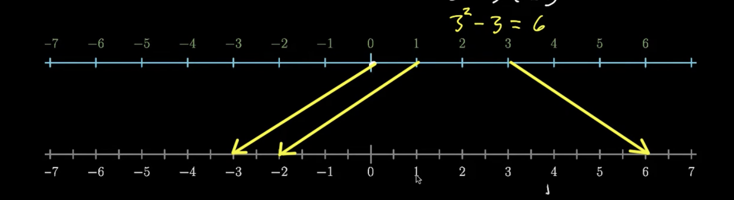
For higher dimensional spaces, we might need to use animation to show how one input space transforms into another.
A fixed point is a point that doesn't "move" when one function is transformed into another. E.g. \(x=1\) is a fixed point of \(x\mapsto x^2\) since \(1^2=1\)
Recall that the derivative measures the rate of change of a function's value relative to a change in the input. Scalar functions only have one argument, so we take the derivative with respect to that. Multivariable functions have multiple input arguments, so we need to reason about that.
A partial derivative measures the rate of change of one of the input variables when all the others are held constant. The \(i\)th partial derivative \(\dfrac{\partial f}{\partial x_i}\) of function \(f(x_1, \dots, x_m) : \mathbb{R}^{m}\to \mathbb{R}\) is the derivative \(\dfrac{\text{d}}{\text{d}t}f(x_1, \dots, x_{i-1}, x_t, x_{i+1}, \dots, x_m)\).
The first-principles definition of the partial derivatives is inherited from the corresponding definition for the regular derivative: for function \(f : \mathbb{R}^{m}\to \mathbb{R}\), the \(i\)th partial derivative is defined as \(\dfrac{\partial f}{\partial x_i}(x_1, \dots, x_i, \dots, x_m):=\displaystyle\lim_{h\to 0}\dfrac{f(x_1, \dots, x_i +h, \dots, x_m) - f(\vec{x})}{h}\)
The second partial derivative \(\dfrac{\partial f^2}{\partial^2 x_i}\) is the application of the operator \(\dfrac{\partial }{\partial x_i}\) twice to the function \(f\). So, \(\dfrac{\partial f^2}{\partial^2 x_i}:= \dfrac{\partial }{\partial x_i}\left(\dfrac{\partial f}{\partial x_i}\right)\).
Since we have more than one variable to work with, we can reason about the "second partial derivative" that we get by taking the partial derivative with respect to one variable, then the other.
Note that there are \(m^2\) combinations for second derivatives; we will need a way to keep track of them all (covered soon). This is an extension of the single-variable \(m=1\) case; there is only one possible second derivative since \(1^2=1\). Looking at the multivariable case lets us know that the number of second partial derivatives "like to scale quadratically".
The gradient \(\nabla f\) of function \(f : \mathbb{R}^{m}\to \mathbb{R}\) is the \(m\)-dimensional vector in containing all the partial derivatives of \(f\). Thus, \(\nabla f := \begin{bmatrix} \dfrac{\partial }{\partial x_1} f \\ \vdots \\ \dfrac{\partial }{\partial x_m} f \end{bmatrix}\) is itself a function.
When evaluated at a given point, the gradient will be a vector in \(\mathbb{R}^m\) that points in the direction in which the rate of change is highest (i.e. the direction of steepest ascent).
The length (\(\ell_2\) norm) of the gradient at a given point describes the general "steepness" of the function at that point.
"The gradient loves to be dotted against other things."
The directional derivative \(\dfrac{\partial }{\partial \vec{v}}f\) of function \(f\) in direction \(\vec{v}\) is the derivative of the slice of \(f\) that coincides with vector \(\vec{v}\). The directional derivative is a linear combination of the components of \(\nabla f\) by \(\vec{v}\), i.e. \(\dfrac{\partial }{\partial \vec{v}}f(\vec{x}) := \langle\nabla f(\vec{x}), \vec{v} \rangle\)
The first-principles definition of the directional derivative inherits from the definition of the partial derivative: \(\dfrac{\partial }{\partial \vec{v}}f(\vec{x}) := \lim\limits_{h\to 0}\dfrac{f(\vec{x} + h \vec{v}) - f(\vec{x})}{n}\).
Note that the magnitude of \(\vec{v}\) does matter; choosing a larger \(\vec{v}\) in the same direction will increase the magnitude of the directional derivative as well. If we are interpreting the directional derivative as a slope, \(\vec{v}\) must be normalized. To compensate, some definitions require normalized \(\vec{v}\), i.e. declare \(\dfrac{\partial }{\partial \vec{v}}f(\vec{x}) := \left\langle\nabla f(\vec{x}), \dfrac{\vec{v}}{\|\vec{v}\|} =: \hat{v}\right\rangle\).
The notion of a directional derivative implies the notion of a "directional function", i.e. the function defined by a slice of \(f\) by an arbitrary plane. We would have \(f_\vec{v}(\vec{x}):=\langle f(\vec{x}), \vec{v} \rangle\).
Given a point, the direction of steepest ascent is some \(\vec{v}\) such that \(\|\vec{v}\|=1\) that maximizes \(\langle\nabla f(\vec{x}), \vec{v}\rangle\), i.e. the directional function with the steepest slope.
The inner product \(\langle\nabla f(\vec{x}), \vec{v}\rangle\) projects the direction \(\vec{v}\) onto the gradient. Since \(\|\vec{v}\|\) is always \(1\), this inner product is largest when \(\vec{v}\) and the gradient are the same direction (by Cauchy-Schwarz). Thus, the gradient is the direction of steepest ascent.
For the same reason, the magnitude of the gradient is the rate of change in the direction of steepest ascent; since "steepness" is determined by the maximal steepness in any direction, this is the steepness of the function.
The parametric curve \(C : \mathbb{R}\to \mathbb{R}^m\) defined by \((f_1(t), \dots, f_m(t))\) for \(t\in [a,b]\) is equivalent to the vector-valued function \(\displaystyle\vec{r}(t)=\sum\limits_{i=0}^{m}f_i(t)\vec{e}_i=\begin{bmatrix} f_1(t) \\ \vdots \\ f_m(t) \end{bmatrix}\in \mathbb{R}^m\).
We differentiate parametric curve by interpreting them as vector-valued functions, taking the gradient of the of the vector-valued function, then re-reinterpreting the gradient as a parametric curve. We can derive by first-principles that this is indeed the derivative of the curve.
Composing a parametrization of a curve with some continuous, bijective function \(g:\mathbb{R}\to \mathbb{R}\) that transforms \(t\) won't change the shape of the curve (and thus the direction of the derivative at any given point), but it will change the magnitude of the derivative at that point.
TLDR: \(\dfrac{\text{d} }{\text{d} t} f(\vec{v}(t)) = {\langle \nabla f(\vec{v}(t)), \dfrac{\text{d} }{\text{d} t}\vec{v}(t)\rangle}\)
Multivariable function composition has an additional wrinkle: functions of different numbers of dimensions can be composed. We can have compositions like \(\mathbb{R}\to \mathbb{R}^{m} \to \mathbb{R}\) that act like single-variable functions, but have a multivariable "hidden layer".
The chain rule(s) are most intuitive when expressed in Leibniz notation, where we can (hand-wavily) interpret the differential \(\text{d}x\) as a "little nudge" in the value of \(x\). We can interpret the single-variable chain rule \(\dfrac{\text{d} y}{\text{d} x} = \dfrac{\text{d} y}{\text{d} u} \dfrac{\text{d} u}{\text{d} x}\) (where \(u\) is a function of \(x\) and \(y\) is a function of \(u\)) as saying that the nudge \(\text{d}x\)'s effect on \(y\) is the nudge \(\text{d}x\)'s effect on \(u\)'s effect on \(y\); the nudge \(\text{d}x\) "propagates" through function \(u\) to affect function \(y\).
In the \(\mathbb{R}\to \mathbb{R}^{2} \to \mathbb{R}\) case, the multivariable chain rule looks like \(\dfrac{\text{d} }{\text{d} t}f(x(t), y(t))=\dfrac{\partial f}{\partial x}\times \dfrac{\text{d} x}{\text{d} t} + \dfrac{\partial f}{\partial y}\times \dfrac{\text{d} y}{\text{d} t}\). We see that the different components of the multivariable function "separate out" into expressions corresponding to each variable that get recombined by addition; these expressions are instances of the single-variable chain rule.
In the general case, the multivariable chain rule states that for \(\vec{v}: \mathbb{R}\to \mathbb{R}^{m}\) and \(f: \mathbb{R}^{m}\to \mathbb{R}\), the derivative of \(f \circ \vec{v} : \mathbb{R}\to \mathbb{R}^{m}\to \mathbb{R}\) is \({\langle \nabla f(\vec{v}(t)), \dfrac{\text{d} }{\text{d} t}\vec{v}(t)\rangle}\).
This formula looks quite a bit like a directional derivative; the directional derivative is a special case of the chain rule where the inner function (\(\vec{v}(t)\)) is a function with constant \(\vec{v}'(t)\), i.e. a line in a particular direction.
Note that the multiplication in \(\dfrac{\text{d} }{\text{d} x} f(g(x)) = f'(g(x)) \cdot g(x)\) generalizes to the inner product in the multidimensional case.
We know \(\dfrac{\text{d} }{\text{d} t} \vec{v}(t)=\lim\limits_{h\to 0}\dfrac{\vec{v}(t+h)-\vec{v}(t)}{h}\). We can express the limit behavior as an error \(E(h)\) in terms of \(h\), so \(\dfrac{\text{d} }{\text{d} t} \vec{v}(t)=\dfrac{\vec{v}(t+h)-\vec{v}(t)}{h} + E(h)\) and thus \(\dfrac{\text{d} }{\text{d} t} \vec{v}(t) h={\vec{v}(t+h)-\vec{v}(t)} + h \cdot E(h)\). Clearly \(\| h \cdot E(h) \|\in o(h)\), so \(\dfrac{\text{d} }{\text{d} t} \vec{v}(t) h={\vec{v}(t+h)-\vec{v}(t)} + o(h)\). Re-arranging, we get \(\vec{v}(t+h)=\vec{v}(t)+ \dfrac{\text{d} }{\text{d} t} \vec{v}(t)h + o(h)\). Subbing in to the first-principles definition for derivative of the nested function \(f(\vec{v}(x))\), we have \(\dfrac{\text{d} }{\text{d} t}f(\vec{v}(t))=\lim\limits_{h\to 0}\dfrac{f(\vec{v} (t+h))-f(\vec{v}(t))}{h} = \lim\limits_{h\to 0}\dfrac{f(\vec{v}(t) + \dfrac{\text{d} }{\text{d} t} \vec{v}(t)h + o(h)) - f(\vec{v}(t))}{h}\). The \(o(h)\) term is negligible since \(h\to 0\), so we are left with \(\lim\limits_{h\to 0}\dfrac{f(\vec{v}(t) + \dfrac{\text{d} }{\text{d} t} \vec{v}(t)h) - f(\vec{v}(t))}{h} = \dfrac{\partial }{\partial \vec{v}} f(\vec{v}(t))\), i.e. the formal definition of the directional derivative in the direction \(\vec{v}(t)\).
TLDR: \(\kappa(t)=\dfrac{\vec{f}(t)' \times \vec{f}(t)''}{\|\vec{f}(t)'\|^3}=\dfrac{x'(t)y''(t)-y'(t)x''(t)}{(x'(t)^2+y'(t)^2)^{\frac{3}{2}}}\) (in 2D)
In single dimensional calculus, outputs and derivatives can only move around in one dimension. Thus, when we reason about rate of change, rate of rate of change, etc, we are confined to one dimension. Granting two output dimensions opens up access to all the tools of planar geometry; higher-dimensional functions let us use higher-dimensional geometry.
Geometrically, the curvature \(\kappa_t=\dfrac{1}{R_t}\) of a parametric function in \(\mathbb{R}^2\) at time \(t\) is the inverse of the radius \(R\) of the circle tangent to the function at time \(t\). To calculate this, we need to know the size and rate of change of the tangent vector at time \(t\) relative to arc length.
For parametric function \(\vec{f}(t)=(x(t), y(t))\), we define \(\hat{T}(t)\) as the unit tangent vector function and \(s(t)\) as the arc-length function (i.e. the spatial distance travelled at time \(t\) over timestep \(\text{d}t\)). We want to know how much the unit tangent vector is changing relative to some step in space (not time) along the curve. From this, we find \(\kappa_t:=\left\| \dfrac{\text{d} \hat{T}}{\text{d} s}\right\|\).
Note that since we are operating in two dimensions, we want to understand if the change in the tangent vector is happening orthogonally to the tangent vector itself or not. If it's not, the function "accelerates" in the direction it's already going, leading to low curvature. The more orthogonal it is, the curvier the function will be. This foreshadows a cross product in the definition.
Expanding out, we get (as a functional equation) \[\kappa:=\left\| \dfrac{\text{d} \hat{T}}{\text{d} s}\right\| = \dfrac{\left\| \dfrac{\text{d} \hat{T}}{\text{d} t} \right\|}{\left\| \dfrac{\text{d} \vec{f}}{\text{d} s} \right\|} = \dfrac{\left\| \dfrac{\text{d} \hat{T}}{\text{d} t} \right\|}{\| \vec{f}' \|} = \dfrac{\dfrac{\vec{f}'}{\|\vec{f}' \|}\times \dfrac{\vec{f}''}{\| \vec{f}'\|}}{\|\vec{f}'\|}=\dfrac{\vec{f}' \times \vec{f}''}{\|\vec{f}'\|^3}=\dfrac{x'(t)y''(t)-y'(t)x''(t)}{(x'(t)^2+y'(t)^2)^{\frac{3}{2}}}\]
So, \(\kappa(t)=\dfrac{\vec{f}(t)' \times \vec{f}(t)''}{\|\vec{f}(t)'\|^3}=\dfrac{x'(t)y''(t)-y'(t)x''(t)}{(x'(t)^2+y'(t)^2)^{\frac{3}{2}}}\).
A helix (with radius \(1\)) is a parametric curve defined by \(\vec{h}(t)=(\cos(t), \sin(t), \frac{t}{c})\).
So, we see that as \(c\to \infty\), the helix approaches a circle, and thus \(\kappa\to 1\). As \(c\to 0\), the helix approaches a straight line, and thus \(\kappa\to 0\). For any in-between choice of \(c\), we see that \(\kappa < 1\) since the vertical travel of the helix makes it slightly less curved than a circle.
We can reason about orthogonality; how similar (or dissimilar) the directions of two vectors are. In two dimensions, this is a range \([0,1]\); curvature is the (dis)similarity of the directions of the first and second derivatives.
In one dimension, there are only two directions, positive and negative, which are linearly dependent. Thus, the "orthogonality" relationship between two vectors isn't a contiguous range, but a discrete choice \(\set{+, -}\). So, "curvature" is an element in \(\set{+,-}\times \set{+,-}\), where the first element is the first derivative and the second the second.
This is, of course, the second derivative test for concavity. In one dimension, the only meaningful possibilities are whether the first and second derivates have the same sign (convex) or different signs (concave). In higher dimensions, we can measure this relationship with a number.
TLDR: concavity is the 1D special case of curvature.
Curvature is a property of the geometric shape of the plot, so it makes sense that we measure it using arc length. Parametrizations can happen at different speeds; this shouldn't affect the curvature. But tangent lines, concavity, etc. are also geometric properties, and yet to calculate those, we differentiated with respect to the variable directly. What the shit?
The shape of \(y=f(x)\) plots is implicitly described by the parametric function \(g(t)=(t, f(t))\). Since the rate of change of the first argument \(t\) is constant, the arc length is proportional to the change in \(f(t)\) (i.e. \(\dfrac{\text{d} f}{\text{d} t}\)) via the Pythagorean theorem. Further, because our "step-size" \(\text{d}t\) is infinitesimal, arc is almost linearly proportional to \(\dfrac{\text{d} f}{\text{d} t}\), since \(\lim\limits_{b\to 0}\sqrt{a^2+b^2}=a\). Note there is no additional proportionality constant; \(\dfrac{\text{d} f}{\text{d} t}\) approximates the arc length itself.
A vector-valued function is a function whose output is a vector, i.e. a function of the (general) form \(f : \mathbb{R}^{m}\to \mathbb{R}^n\). Here, we need to keep track of \(m\times n\) relationships between input and output variables.
Partial derivatives of vector-valued functions look like partial derivatives of multivariable functions, just with vector outputs. The partial derivative \(\dfrac{\partial \vec{f}}{\partial x_i}\) is a vector describing the "nudge direction" of the output if input variable \(x_i\) is nudged; it is the derivative of the line corresponding to variable \(x_i\) in the output space/surface.
For a vector field, the partial derivative \(\dfrac{\partial \vec{v}}{\partial x_i}\) corresponds to the difference between the vectors before and after being nudged by \(\partial x_i\) in the \(x_i\) direction.
TLDR: \(\text{div}{\, \vec{f}(\vec{x})} = \langle \vec{f}, \nabla{\vec{f}} \rangle = \vec{f}\cdot \nabla\)
We can visualize vector fields by imagining what fluid flow would look like if particles followed their position's vector at each time step. Under this interpretation, we might wonder if the density of the fluid flowing through a point or region of the field stays constant or not. If it doesn't, is the density increasing (indicating a sink), or decreasing (indicating a source)?
In a 1D, if divergence of the function \(f\) about point \(t\) is positive, more fluid is leaving than entering, so the rate of change is faster in the positive direction than the negative one, and thus the partial derivative \(\dfrac{\partial f}{\partial x}(t)\) is positive.
Clearly, this is true for any single dimension of a multi-dimensional function, so the general definition will combine these. Divergence should be higher if the function diverges more in more directions. Summing all the partial derivatives leads to this asymptotic behavior.
Note: for actual 2D fluid flow, divergence must be \(0\) everywhere since matter cannot be created or destroyed. The Navier-Stokes equations describe the rules of fluid flow; \(\text{div}{\, F}=\vec{0}\) is one of them.
Divergence \(\text{div}{} : \mathbb{R}^{m}\to \mathbb{R}\) is a scalar-valued differential operator that measures the change in density about a given point in a vector field.
In the vector field \(\vec{v}: \mathbb{R}^{2}\to \mathbb{R}^2\) case, \(\text{div}\,{\vec{v}(x,y)}=\dfrac{\partial }{\partial x}P + \dfrac{\partial }{\partial y}Q\)
In the general case \(\vec{f} : \mathbb{R}^{m}\to \mathbb{R}^n\) where \(\vec{f}\) is described by \((f_1(\vec{x}), \dots, f_m(\vec{x}))\), we have \(\text{div}{\, \vec{f}(\vec{x})} = \langle \vec{f}, \nabla{\vec{f}} \rangle\) (i.e. \(= \vec{f}\cdot \nabla\))
TLDR: \(\text{curl}{\, \vec{v}(\vec{x})} = \nabla\times \vec{v}\). In 3D, \(\text{curl}{\, \vec{v}(\vec{x})}=\dfrac{\partial Q}{\partial x} -\dfrac{\partial P}{\partial y}\). In 3D, \(\text{curl}{\, \vec{v}(\vec{x})}=\left( \dfrac{\partial R}{\partial y} - \dfrac{\partial Q}{\partial z} \right) \hat{i} + \left( \dfrac{\partial P}{\partial z} - \dfrac{\partial R}{\partial x} \right) \hat{j} + \left( \dfrac{\partial Q}{\partial x} - \dfrac{\partial P}{\partial y} \right) \hat{k}\)
Again, we use out "fluid-flow" model of vector fields. Curl describes the direction of rotation around a given point. One can think of (2D) curl as describing the behavior of a twig anchored at a given point; will the twig rotate clockwise, counter-clockwise, or stay still? How fast will it rotate?
If the vector field is "rotating" around a point, for any axial direction, the vectors on either side of the point (along the axis) should be pointing in roughly different directions. Thus, the directional derivative corresponding to the axis' direction should be "significantly" positive or negative.
By looking at the directional derivative along "enough" axes, we should be able to determine the overall rotational behavior around our point. It turns out that it is enough (and most convenient) to simply check each partial derivative at the point.
In 2D, a "perfect" counter-clockwise rotation would have \(\dfrac{\partial Q}{\partial x} > 0\) and \(\dfrac{\partial P}{\partial y}<0\). This should have the strongest curl possible. Defining curl as \(\dfrac{\partial Q}{\partial x} -\dfrac{\partial P}{\partial y}\) maximizes this. Seems reasonable.
Much like direction, in 2D, there are only two rotational directions: clockwise and counter-clockwise. But clearly, there's infinitely more "space" in which to rotate in 3D. We can describe 3D rotation by a single vector: it points in the direction of the axis of rotation, and its magnitude indicates the speed of rotation.
We know that rotation corresponds to orthogonality; in linear algebra, the orthogonal matrices completely describe rotations. Any plane coinciding with an axis of rotation will be orthogonal to the direction of rotation at points of intersection. We know the cross product produces an orthogonal vector given two other vectors; thus, we should expect a cross product to come up in the general definition of curl.
Curl \(\text{curl}\,:\mathbb{R}^{m}\to \mathbb{R}\) is a scalar-valued differential operator that measures the rotation around a given point in a vector field.e
In the 2D case, curl is given by \(\text{curl}{\, \vec{v}(x,y)}=\dfrac{\partial Q}{\partial x} - \dfrac{\partial P}{\partial y}\).
In the 3D case, curl is (formally) given by \(\text{curl}{\, \vec{v}(x,y,z)}=\det{\begin{bmatrix} \hat{i} & \hat{j} & \hat{k} \\ \dfrac{\partial }{\partial x} & \dfrac{\partial }{\partial y} & \dfrac{\partial }{\partial z} \\ P & Q & R\end{bmatrix}}\). What?
The Laplacian \(\nabla^{2}\) (or \(\Delta\)) \(: \mathbb{R}^{m}\to \mathbb{R}\) is a differential operator that measures how "extremal" a function \(f\) is at a given point \(\vec{x}\); it is very positive at "maximal" areas and very negative in "minimal" areas.
In the scalar calculus case, we only have one output dimension, so the property of being extremal at a point is boolean: either it is or it isn't. But, with multiple output dimensions, a point may be extremal in one (or more) dimension but not in the others. So, points can be "kind of" extremal in the way that the slope of a multivariable function can be "kinda" steep. Thus suggests that "extramalness" is now measured in \(\mathbb{R}\) and involves directionality.
If a point is very extremal, the slope around that point should be either strongly away from that point (maximal) or towards that point (minimal). Thus, the laplacian is the divergence of the gradient.
We have \(\text{div}{\, \text{grad}{\, f}}=\text{div}{\, \nabla{f}}=\nabla\cdot \nabla f = \nabla^{2} f\). So, the notation for the laplacian operator is \(\nabla^2\). Expanding the dot product, we find for \(f: \mathbb{R}^{m}\to \mathbb{R}^n\), \(\nabla \cdot \nabla f=\displaystyle\sum\limits_{i=1}^{m} \dfrac{\partial^{2}f}{\partial x_i}\).
A harmonic function is a function whose laplacian is \(0\) everywhere, i.e. \(f\) is harmonic if \(\nabla^{2}f=0\).
In one dimension, the laplacian is the second derivative, so a function is harmonic iff the second derivative is \(0\) \(\implies\) the first derivative is constant \(\implies\) the function is linear. Thus, the only harmonic functions \(\mathbb{R}\to \mathbb{R}\) are lines. However, in higher dimensions, the laplacian "averages" all the directions; directional derivatives may be positive or negative, as long as they "cancel out".
Harmonic functions are beasts from the kingdom of differential equations. They come up as "stable points" where a function defines values at a point as an "average" of the values around that point.
The set of harmonic functions on open set \(U\) is the kernel of \(\nabla^{2}\). Since \(\nabla^{2}\) is a linear operator, \(\ker{\nabla^{2}}\) is a subspace (reasoning) of the vector space of functions; linear combinations of harmonic functions are also harmonic.
We say differentiable functions are locally linear. Differentiable scalar functions can be approximated around any point by a tangent line. In the general case, a differentiable multivariate function can be approximated around any point by a tangent hyperplane.
If we think of multivariate functions of the form \(\mathbb{R}^{k}\to \mathbb{R}^{k}\) as transformations of space, the tangent hyperplane is a linear approximation of the transformation the function applies around that point. Linear transformations are uniquely and totally defined by matrices, this transformation is described by a \(k\times k\) matrix called the Jacobian.
The Jacobian \(J\) is a functional operator \(J : (\mathbb{R}^{k}\to \mathbb{R}^{k}) \to (\mathbb{R}^{k}\to \mathbb{R}^{k\times k})\) that describes the linear approximation of a \(\mathbb{R}^{k}\to \mathbb{R}^k\) function. Specifically, for function \(\vec{f}(\vec{x})=\begin{bmatrix} f_1(\vec{x}) \\ \vdots \\ f_k(\vec{x}) \end{bmatrix}\), we have \(J_{\vec{f}}(\vec{x})=\begin{bmatrix} \dfrac{\partial f_1 }{\partial x_1} & \dots & \dfrac{\partial f_k }{\partial x_1} \\ \vdots & \ddots & \vdots \\ \dfrac{\partial f_1}{\partial x_k} & \dots & \dfrac{\partial f_k}{\partial x_k}\end{bmatrix}\). The \((i,j)\)th entry describes the effect of a nudge on the \(i\)th argument on the \(j\)th output component.
For point \(\vec{x}\), the value \(\det{J_\vec{f}(\vec{x})}\) describes, in a scalar quantity, how much the transformation around point \(\vec{x}\) expands and contracts space. If we think of infinitesimally small unit square rooted at point \(\vec{x}\), the same square in the output space (now rooted at \(\vec{f}(\vec{x})\)) will have area \(\det{J_\vec{f}(\vec{x})}\).
TLDR: \(L(\vec{p})=[\nabla f](\vec{p})\cdot(\vec{p}-\vec{p}_0)+f(\vec{p}_0)\)
Differentiable functions \(\mathbb{R}\to \mathbb{R}\) have tangent lines at each point, which linearly approximate the behavior of the function around that point. Differentiable functions \(\mathbb{R}^{m}\to \mathbb{R}\) have analogous tangent hyperplanes that approximate the behavior of the function around a given point.
We can formalize this as a linearization function \(L:(\mathbb{R}^{m}\to \mathbb{R})\times \mathbb{R}^{m}\to \mathbb{R}^{m}\) that takes a function and a point in that function's domain and returns the tangent plane at that point.
Much like tangent lines, tangent hyperplanes are linear approximations of a function around a point. It is not much harder to take a derivative (and then a linear approximation) of a function than to evaluate the function, and it is much easier to evaluate the linear approximation. Thus, if a function needs to be sampled many times around a point, a linear approximation is practically as good at a fraction of the cost.
TLDR: \(L(x,y)= x'(x-x_0) + y'(y-y_0)+z_0\)
How do we even describe a 2D plane embedded in a 3D space?
So, each planar "slice" of a plane is a line (of the form \(mx_i +b\)), so both partial derivatives of the plane are constant. More generally, the gradient is constant everywhere on the plane.
Let 2D plane \(L\) is at height \(z_0\) at some point \((x_0,y_0)\) in the input space, and record \(x' := \dfrac{\partial L}{\partial x}\) and \(y':=\dfrac{\partial L}{\partial y}\). Then, we can figure out the height of the plane at any point by "measuring the offset from \((x,y)\)". Specifically, we get \(L(x,y)= x'(x-x_0) + y'(y-y_0)+z_0\). In "homogeneous form", this plane is described by \(x'(x-x_0) + y'(y-y_0)=0\).
We want to find the tangent plane of function \(f:\mathbb{R}^{2}\to \mathbb{R}\) at point \(\vec{p}\in \mathbb{R}^2\).
Plugging into the formula, we find the equation of the tangent plane as \(L(x,y)=\left(\dfrac{\partial f}{\partial x}(x,y)\right)(x-x_0) + \left(\dfrac{\partial f}{\partial y}(x,y)\right)(y-y_0)+f(x,y)\)
Again, we can generalize this as a dot product between the gradient at the point and a vector of expressions of the form \(a-a_0\): the tangent plane at point \(\vec{p}\) is described by \(L(\vec{p})=[\nabla f](\vec{p})\cdot(\vec{p}-\vec{p}_0)+f(\vec{p}_0)\).
TLDR:
Let's use the rest of the Taylor series, eh? Like in the single variable case, adding more and more terms of the function's Taylor series gives a better and better approximation.
A quadratic approximation is a conic section, i.e. has the form \(Q(x,y)=a+bx+cy+dx^{2}+exy +fy^2\) (all polynomial terms of order \(\leq 2\) from basis \(\set{1, x, y}\)). A linear (technically, affine) approximation uses just the first derivative; a quadratic approximation takes the second derivative into account as well.
So, we want \(\dfrac{\partial^{2}Q}{\partial x^2}(x_0,y_0)=\dfrac{\partial^{2}f}{\partial x^{2}}(x_0,y_0)\), \(\dfrac{\partial^{2}Q}{\partial x \partial y}(x_0,y_0)=\dfrac{\partial^{2}f}{\partial x \partial y}(x_0,y_0)\), and \(\dfrac{\partial^{2}Q}{\partial y^2}(x_0,y_0)=\dfrac{\partial^{2}Q}{\partial y^{2}}(x_0,y_0)\). Note that we already have \(L\) as an approximation of \(f\) around \((x_0, y_0)\) that we can use for the non-quadratic terms, giving \(Q(x,y)=L(x,y)+a(x-x_0)^{2}+b(x-x_0)(y-y_0)+c(y-y_0)^2\). For each of the \(3\) partial derivatives, we expand like \(\dfrac{\partial^{2} Q}{\partial x^2}=\dfrac{\partial }{\partial x}\left( \dfrac{\partial }{\partial x} Q(x,y) \right) =\dfrac{\partial }{\partial x}(f_x(x_0, y_0)+2a(x-x_0)+b(y-y_0))=2a\), which gives us \(3\) respective constants: \(\dfrac{\partial^{2} Q}{\partial x^2}=2a\), \(\dfrac{\partial^{2} Q}{\partial x \partial y}=b\), \(\dfrac{\partial^{2} Q}{\partial y^2}=2c\).
So, the full quadratic approximation is \(Q(x,y)=L(x,y) + \dfrac{1}{2}{\dfrac{\partial^{2}f}{\partial x^2}}(x-x_0)^{2} + \dfrac{\partial^{2}f}{\partial x \partial y}(x-x_0)(y-y_0)+\dfrac{1}{2}\dfrac{\partial^{2} f}{\partial y^2}(y-y_0)^{2}\).
The Hessian matrix \(H_f\in \mathbb{R}^{m\times m}\) of twice-differentiable function \(f : \mathbb{R}\to \mathbb{R}^{m}\) contains all the second derivatives of \(f\); it is defined by \(H_f := \begin{bmatrix} \dfrac{\partial^{2}f}{\partial x_1^{2}} & \dots & \dfrac{\partial^{2}f}{\partial x_1 \partial x_m} \\ \vdots & \ddots & \vdots \\ \dfrac{\partial^{2}f}{\partial x_m \partial x_1} & \dots & \dfrac{\partial^{2}f}{\partial x_m^{2}} \end{bmatrix}\). We can think of the Hessian as a functional operator \(H : (\mathbb{R}\to \mathbb{R}^{m})\to (\mathbb{R}^{m}\to \mathbb{R}^{m\times m})\); the Hessian is a matrix of functions.
To perform the equivalent of the "second derivative test" for functions \(\mathbb{R}\to \mathbb{R}^m\), we take the determinant of the Hessian. For example, if \(\det{H_f(c)}>0\) and \(\dfrac{\partial^2 f}{\partial x^2} (c)>0\) at point \(c\), then \(f\) is concave (up) at point \(c\).
A quadratic form is an expression of exclusively quadratic terms, usually of multiple variables, e.g. \(ax^{2}+bxy + cy^2\). Quadratic forms can be expressed idiomatically using matrix multiplication: \(ax^{2}+bxy + cy^2\) is equal to the matrix product \(\begin{bmatrix} x & y \end{bmatrix}\begin{bmatrix} a & b/2 \\ b/2 & c \end{bmatrix}\begin{bmatrix} x \\ y \end{bmatrix}\). So, if \(\vec{\phi}\) is a polynomial basis, a quadratic form can be expressed as \(\vec{\phi}^\top M \vec{\phi}\).
Quadratic forms are the convenient "vector expression" for quadratic expressions in the same way that the dot product is the convenient "vector expression" for a linear expression (linear combination).
We can express our quadratic approximation using a quadratic form where the Hessian is the middle matrix and \((\vec{x}-\vec{x}_0)\) is the vector. We have \(Q(\vec{x})=f(\vec{x}_0)+\nabla f(\vec{x})\cdot (\vec{x}-\vec{x}_0) + \dfrac{1}{2}(\vec{x}-\vec{x}_0)^{\top}H_f(\vec{x}_0)(\vec{x}-\vec{x}_0)\).
It is useful to find inputs to multivariable functions that yield maximal and maximum values. Formally, for function \(f:\mathbb{R}^{m}\to \mathbb{R}\), we want to find \(\arg\max\limits_{\vec{x}\in \mathbb{R}^{m}}f(\vec{x})=\arg\min\limits_{\vec{x}\in \mathbb{R}^{m}}-f(\vec{x})\). On well-behaved functions, this must occur when each variable is at a maximum, i.e. where \(\nabla f=\vec{0}\), a critical point. This is an equality; we analytically solve for critical points, just like in the single-variable case.
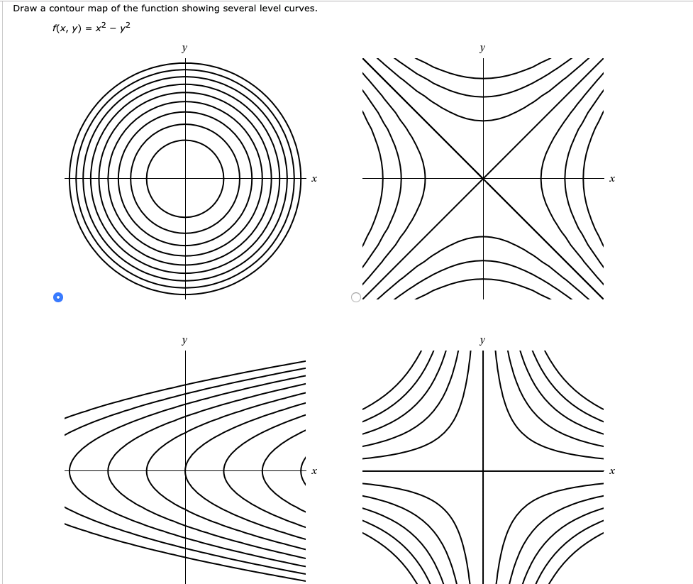
However, functions may have critical points that aren't maximal or minimal, i.e. saddle points. E.g. the pringle-shaped function \(f(x,y)=x^{2}-y^{2}\) has a saddle point at the origin: \((0,0)\) is a minimum of \(f_x\) but a maximum of \(f_y\).
In single-variable calculus, the second derivative at a critical point tells us whether it is a maximum, minimum, or something else (like \(f(0)\) for \(f(x)=x^{3}\)). Currently, the closest multivariable equivalent we have is curvature. But this is a vector; vectors in \(\mathbb{R}^{m}\) for \(m>1\) cannot be assigned a total order, so we can't compare it to \(\vec{0}\) or whatever. We need some function \(\mathbb{R}^{m}\to \mathbb{R}\) parametrized by \(f\) that "preserves positivity" somehow.
We compute the quantity \(h:=\dfrac{\partial^2 f}{\partial x^2}(x_0, y_0)\dfrac{\partial^2 f}{\partial y^{2}}(x_0, y_0)-\left[\dfrac{\partial^2 f}{\partial x \partial y}(x_0, y_0)\right]^{2}\) for critical point \((x_0, y_0)\).
Intuitively, \(\dfrac{\partial^2 f}{\partial x^2}(x_0, y_0)\dfrac{\partial^2 f}{\partial y^{2}}(x_0, y_0)\) is positive when the concavity is the same in both the \(x\) and \(y\) directions; both are either concave or convex. Its absolute value measures how much the concavities "agree". \(\left[\dfrac{\partial^2 f}{\partial x \partial y}(x_0, y_0)\right]^{2}\) measures how much the function \(f\) looks like \((x,y)\mapsto xy\), which is the "canonical saddle"; it accounts for "saddling" that might occur in other directions than pure \(x\) and \(y\). So, critical points that resemble saddles will be negative and critical points that don't will be positive.
Sometimes, particularly in high dimensions, solving for maxima/minima analytically is prohibitively difficult; numerical methods are required. A popular method (well-known in machine learning) is to pick a random point and move in the direction of steepest descent to find a local minimum. This corresponds to iterating the equation \(\vec{x} \leftarrow \vec{x}-\eta \nabla f(\vec{x})\) for (random) initial choice \(\vec{x}\) and learning distance \(\eta\).
TLDR:
A constrained optimization problem is an optimization problem where a constraint (set of allowed values for input arguments) is placed on the space of possible arguments.
The constraint set is usually described by an equation or inequation whose solutions comprise the elements of the set. This equation has the same input arguments as the function, and thus exists in the same space. Thus, we can think of optimizing along the curve defined by that constraint.
This constraint equation will look like \(c(\vec{x})=a\) or \(c(\vec{x})>a\), e.g. \(x^{2}+y^{2}=1\). If the function \(f\) we are optimizing maps \(\mathbb{R}^{m}\to \mathbb{R}\), the set \(c\) describes in \(\mathbb{R}^{m}\) will be (hand-wavingly) an embedding of an \(m-1\) dimensional curve, since one variable can be brought to the other side of the equation and defined in terms of the other ones. We can also view the constraint as the isoline with value \(a\) of the function \(c:\mathbb{R}^{m}\to \mathbb{R}\).
If we plot the isolines the function \(f\) and the constraint, we will find that \(c\) will be tangent to the isoline of \(f\) corresponding to the optimization solution. Viewing the constraint as isoline \(a\) of \(c(\vec{x})\), we know that two functions have tangent isolines at a point iff their gradient has the same direction at that point. This lets is express the solution algebraically.
Let \(f:\mathbb{R}^{m}\to \mathbb{R}\) be a function we are optimizing (maximizing) subject to constraint \(c(\vec{x})=a\) for \(c: \mathbb{R}^{m}\to \mathbb{R}\). At the true optimal point \(\star{\vec{x}}\), the gradients of \(f\) and \(c\) point in the same direction. So, we have \(\nabla f = \lambda \nabla c\) for Lagrange multiplier \(\lambda\in \mathbb{R}\).
This yields a system of equations with \(m\) equations and \(m+1\) unknowns, including \(\lambda\). We can solve for all the variables by adding \(c(\vec{x})=a\) to our system of equations.
We can interpret \(\lambda\) as a measure of how quickly nudges to the height of the constraint isoline affect the optimal value; we have \(\star{\lambda}=\dfrac{\text{d} {\star{\vec{x}}}}{\text{d} a}\) (proof), where \(\star{\lambda}\) is the value of \(\lambda\) corresponding to the optimal solution \(\star{\vec{x}}\).
Given a function \(f:\mathbb{R}^{m}\to \mathbb{R}\) to optimize along constraint \(c(\vec{x})=a\) for \(c: \mathbb{R}^{m}\to \mathbb{R}\), we define the corresponding Lagrangian \(\mathcal{L}: \mathbb{R}^{m+1}\times \mathbb{R}\to \mathbb{R}\) as \(\mathcal{L}(\dots\vec{x}, \lambda)=f(\vec{x})-\lambda(c(\vec{x})-a)\), which repurposes the Lagrange multiplier expression into a function. This encodes our constrained optimization problem as an unconstrained optimization problem: solving \(\nabla \mathcal{L}=\vec{0}\) yields our solution.
Note that \(\nabla \mathcal{L}=\vec{0}\) may yield non-optimal solutions; all must be plugged back into the original function and compared. The solution that corresponds to the original constrained optimization will be a saddle point of \(\mathcal{L}\).
in modern terms:
The derivative is a linear map between tangent spaces:
D(f \circ g)x = Df{g(x)} \circ Dg_x
This is literally composition of linear maps.
"nudge model" of differentials, just talking about differentials on their own like \(\text{d}x\)
intuition for exponential functions: the traditional exponential means speed up is wrong. in the purest form, an expoentnial function is a function where the rate of change is a function of (proportional to) the current location.
a lot of the time, we construct a scalar measure of something out of a bunch of vector derivatives (laplacian, divergence, 2D curl, etc). A few things
TLDRs become definition boxes
Multivariable calculus is straightforward generalization of single-variable calculus concepts to multiple dimensions. And yet, it enables any expression can be interpreted as a multivariable function and thrown to the hounds of calculus.