Chapter 2 - Introduction to Probabilistic Modeling
Probability is the extension of logic from the discrete to the continuous
Probability Theory and Random Variables
An experiment has an outcome (in the outcome space). An event is a meaningful set of outcomes. Probabilities about events are expressed as random variables\(X\), which has its own outcome space\(\mathcal{X}\).
E.g. a die roll is an experiment, rolling a \(1\) is an outcome, rolling an even number is an event. We may define \(X\) as the outcome of a die roll, then compute things like \(P(X > 3)\) that correspond to events.
Defining Distributions
Discrete Distributions and PMFs
A probability mass function (PMF) is a function \(p : \mathcal{X}\to[0,1]\) where \(\displaystyle\sum\limits_{x\in\mathcal{X}}p(x)=1\); it describes the probability of a particular outcome\(\mathcal{x}\in\mathcal{X}\) occurring
We must have \(\displaystyle\sum\limits_{x\in\mathcal{X}}p(x)=1\) because the probability of an outcome being measured from an experiment is by definition \(1\)
\(P(X\in A) = \displaystyle\sum\limits_{x\in A}p(x)\) where \(A \subseteq \mathcal{X}\) is an event
The Bernoulli distribution describes an experiment; it as a single parameter\(\alpha\) that defines the probability of the experiment succeeding.
Compactly, we write its PDF as \(p(x)=\alpha^x(1-\alpha)^{1-x}\)
The (discrete) uniform distribution describes the distribution where every outcome is equally likely to occur.
For \(\mathcal{X}\) where \(\#\mathcal{X}=n\), its PDF is \(p(x)=\dfrac{1}{n}\)
The poisson distribution describes the probability of a certain number of incidents occurring (over an implicitly finite timespan). Its parameter \(\lambda\) is the expected number of incidents in the timeframe.
Its PDF is \(p(x)=\dfrac{\lambda^{x}e^{-\lambda}}{x!}\)
Note: although the distribution seems to act like a rate, the actual length of time being measured cancels out, so there is no parameter to define the "time" events are measured over
Continuous Distributions and PDFs
The continuous analog to the PMF is the probability density function (PDF), defined as a function \(p : \mathcal{X}\to [0, \infty)\) where \(\displaystyle\int_{\mathcal{X}}p(x)\,dx=1\)
It is used similarly to a PMF, but evaluating it at any point is meaningless because the probability of a particular outcome happening over an experiment defined by a continuous distribution is \(0\). It measures the "density", something more fuzzy.
\(P(X\in A)=\displaystyle\int_{A}p(x)\,dx\)
The continuous uniform distribution is the continuous analog to the discrete uniform distribution; it has PDF \(p(x)=\dfrac{1}{b-a}\) where \(a\) and \(b\) define the bounds of the uniform range.
The exponential distribution is the continuous analog to the poisson distribution and is defined over \(\mathcal{X}=(0, \infty)\) as \(p(x)=\lambda e^{-\lambda x}\) with parameter \(\lambda\).
The Gaussian distribution or normal distribution defines many natural phenomena, as well as the emergent distribution of sample averages of not necessarily Gaussian populations (central limit theorem, roughly).
We have \(p(x)=\dfrac{1}{\sqrt{2\pi \sigma^2}}e^{-\frac{1}{2\sigma^2}(x-\mu)^2}\), but this is not often integrated on directly
Parameters: mean \(\mu\), variance \(\sigma^2\) (derived from standard deviation \(\sigma\)).
This is regarded as the most important distribution due to the central limit theorem
The Laplace distribution is similar to the Gaussian, but more peaked around the mean. It is defined as \(p(x)=\dfrac{1}{2b}e^{- \frac{1}{b}|x-\mu|}\) with parameters \(\mu \in \mathbb{R}\) and \(b > 0\).
The Gamma distribution is the continuous analog to the poisson distribution and is defined over \(\mathcal{X}=(0, \infty)\) as \(p(x)=\dfrac{\beta^\alpha}{\Gamma(\alpha)}x^{\alpha-1}e^{-\beta x}\) (where \(\Gamma(x)\) is the gamma function)
Multivariate Random Variables
Joint Distributions
We define the joint probability mass function \(p:\mathcal{X}\times\mathcal{Y}\to[0, 1]\) and corresponding joint probability distribution \(P\) such that \(p(x, y):=P(X=x, Y=y)\) for random variables \(X\) and \(Y\) with outcome spaces \(\mathcal{X}\) and \(\mathcal{Y}\), respectively.
The PMF must satisfy \(\displaystyle \sum\limits_{x\in \mathcal{X}}\sum\limits_{y\in \mathcal{Y}}p(x, y)=1\)
\(Z=(X, Y)\) is a multivariate random variable with outcome space \(\mathcal{Z=X\times Y}\)
\(d\)-dimensional Random Variables
We generalize joint distributions to \(d\) dimension: we consider a \(d\)-dimensional random variable\(\vec{X}=(X_1, X_2, \dots, X_d)\) with vector-valued outcomes \(\vec{x}=(x_1, x_2, \dots, x_d)\) where each \(x_i\) is chosen from some corresponding outcome space \(\mathcal{X}_i\).
Then, any \(p:\mathcal{X}_1\times \mathcal{X}_2 \times \dots \times \mathcal{X}_d \to [0, 1]\) is a multidimensional probability mass function if \(\displaystyle \sum\limits_{x_1\in \mathcal{X}_2}\sum\limits_{x_2\in \mathcal{X}_2}\dots \sum\limits_{x_d\in \mathcal{X}_d} p(x_1, x_2, \dots, x_d)=1\), or in the continuous case, a multidimensional probability density function if \(\displaystyle\int_{\mathcal{X}_1}\displaystyle\int_{\mathcal{X}_2}\dots \displaystyle\int_{\mathcal{X}_d}p(x_1, x_2, \dots, x_d) \, dx_1 dx_2\dots dx_d=1\)
Marginal Distributions
A marginal distribution of a subset of \(\vec{X}\cong \set{X_1, X_2, \dots, X_d}\supset A\) is found by summing/integrating over the remaining variables \(\set{X_1, X_2, \dots, X_d}\setminus A\).
E.g. the marginal distribution of \(X\) for the \(d=3\) distribution \((X, Y, Z)\) is \(\displaystyle p(x):=\sum\limits_{y\in \mathcal{Y}}\sum\limits_{z\in \mathcal{Z}}p(x, y, z)\); we are summing over the variables \(X, Y\)
Of course, we integrate in the continuous case
Notice how this is still a function: since we are summing/integrating over the variables not in our subset, their degrees of freedom remain, and we get another function
Conditional Probability
We define the conditional probability \(p(y|x)\) of \(X\) given \(Y\) as \(p(y|x):=\dfrac{p(x, y)}{p(x)}\) where \(p(x)>0\)
This is interpreted as the probability that \(Y=y\) given that we know \(X=x\). Hence, "conditional".
Product Rule: \(p(x, y)=p(x|y)p(y)=p(y|x)p(x)\)
This generalizes to the chain rule: \(p(x_1, \dots, x_d)=p(x_1)\displaystyle\prod_{i=2}^{d}p(x_i|[x_1, \dots, x_{i-1}])\)
E.g. \(p(x, y, z)=p(x|[y, z])\times p(y|z)\times p(z)\)
Bayes' Rule: \(p(x|y)=\dfrac{p(y|x)p(x)}{p(y)}\) (follows directly from the product rule)
Variables \(X\) and \(Y\) are independent if \(p(x_1, x_2, \dots, x_d)=p(x_1)p(x_2)\dots p(x_d)\), i.e. if the conditional and marginal distributions are the same. Thus, the variables don't "affect" each other.
Conditional independence and "regular" independence do not imply each other!
Expectations and Moments
Expected Value
The expected value\(\mathbb{E}[X]\) of random variable \(X\) is the average of \(n\to \infty\) samples of \(X\). Numerically, for discrete \(X\), \(\mathbb{E}[X]:=\displaystyle\sum\limits_{x\in\mathcal{X}}x p(x)\) and for continuous \(X\), \(\mathbb{E}[X]:=\displaystyle\int\limits_{\mathcal{X}} x p(x) \, dx\)
We can find the expected value of functions on \(X\) (moments); we have for discrete \(f(X)\)\(\mathbb{E}[f(X)]=\displaystyle\sum\limits_{x\in\mathcal{X}}f(x) p(x)\) and for continuous \(f(X)\)\(\mathbb{E}[f(X)]=\displaystyle\int\limits_{\mathcal{X}} f(x) p(x) \, dx\). We are essentially creating a new random variable named \(f(X)\), then computing the expected value of that.
We can extend expectation to the other types of distributions we've seen (we only write the body of the expression expectation expression for brevity)
Conditional expectation: \(\mathbb{E}[f(Y)|X=x]\approx: f(y)p(y|x)\) collected over \(y\)
Joint expectation, one variable fixed: \(\mathbb{E}[f(X, Y)]:\approx f(x, y)p(x|y)\)
Joint expectation, no variables fixed: \(\mathbb{E}[f(X, Y)]:\approx p(y)\mathbb{E}[f(X, y)]\), i.e. we simply fix the last variable and look at the expectation again
Law of total expectation: \(\mathbb{E}[Y]=\mathbb{E}[\mathbb{E}[Y|X]]\) (the outer expectation is over \(X\), the inner over \(Y\)).
Intuitively, the dependence in the inner expectation gets "averaged out" by the outer expression
Variance
We define the variance\(\text{Var}[X]\) of random variable \(X\) as \(\text{Var}[X] := \mathbb{E}[(X-\mathbb{E}[X])^2]\). This measures how "concentrated" the distribution of \(X\) is around its mean
This interpretation follows from the definition directly; we are measuring the expected euclidean distance of a given instance of \(X\) from its expected value.
Variance is always \(\geq 0\)
Aside: Covariance satisfies the metric axioms, so it is a metric function (distance function) over the space of distributions.
Covariance
Just as variance measures the "spread" of a single variable, covariance\(\text{Cov}[X, Y]\) of \(X\) and \(Y\) measures how spread out two variables are, as well as how spread out their "union" is. We have \(\text{Cov}[X, Y]:=\mathbb{E}[(X-\mathbb{E}[X])(Y-\mathbb{E}[Y])]=\mathbb{E}[XY]-\mathbb{E}[X]\mathbb{E}[Y]\)
We define the correlation\(\text{Corr}[X, Y]\) of \(X\) and \(Y\) as a normalized version of variance that measures how related the two variables are. We have \(\text{Corr}[X, Y]:\dfrac{\text{Cov}[X, Y]}{\sqrt{\text{Var}[X]}\sqrt{\text{Var}[Y]}}\in [-1, 1]\)
\(X\) and \(Y\) are independent if their covariance is \(0\).
We have \(\text{Cov}[X, X]=\text{Var}[X]\)
Here, we are normalizing using the variance of \(X\) and \(Y\)
Properties of Variance and Covariance
Properties of Variance and Covariance
Properties
For random variables \(X, Y\) and \(c\in \mathbb{R}\), the following hold
\(\mathbb{E}[cX]=c\mathbb{E}[X]\)
\(\mathbb{E}[X+Y]=\mathbb{E}[X]+\mathbb{E}[Y]\) (linearity of expectation)
\(\mathbb{E}[XY]=\mathbb{E}[X]\mathbb{E}[Y]\) for any data points
\(\text{Var}[X+Y]=\text{Var}[X]+\text{Var}[Y]\)
\(\text{Cov}[X, Y]=0\)
Extra: (more) Formal Probability Theory
In probability theory, an experiment has an outcome\(\omega\); all the possible outcomes form the outcome space/sample space\(\Omega\). An event is a set of outcomes that denote a "type of thing"; these form the event space\(\mathcal{E} \subseteq \mathcal{P}(\Omega)\) of the experiment.
E.g. rolling a die is an experiment with outcome space \(\set{1, 2, 3, 4, 5, 6}\), so rolling a \(1\) is a possible outcome, whereas rolling an even number is an event corresponding to outcomes \(\set{2, 4, 6}\)
The concept of a random variable is a formalization and generalization of the notion of an experiment on which we can define probabilistic questions.
Axioms of Probability (Appendix)
\((\Omega, \mathcal{E})\) is a measurable space if the outcome space/sample space\(\Omega\) is non-empty and the event space\(\mathcal{E} \subseteq \mathcal{P}(\Omega)\) has the following properties
A probability measure/probability distribution\(P : \mathcal{E} \to [0, 1]\) must satisfy the axioms of probability:
\(P(\Omega) = 1\)
\(A_1, A_2, \dots \in \mathcal{E}\) and \(A_i \cap A_j = \emptyset\) for all \(i, j\)\(\implies\)\(\displaystyle P\left(\bigcup_{i=1}^{\infty}A_i\right) = \sum\limits_{i=1}^{\infty}P(A_i)\)
\((\Omega, \mathcal{E}, P)\) is a probability space/probability measure if all the above properties are true.
A random variable is a function \(X : \Omega \to \mathcal{X}\) that defines a transformation between experiment's probability space and its own probability space; it defines the probability space \((\mathcal{X}, \mathcal{E}_X, P_X)\)
E.g. for a dice roll, \(X\) may represent whether the value is even or odd; this random variable maps \((\set{1, 2, 3, 4, 5, 6}, \mathcal{P}(\Omega), P)\) to \((\set{\text{even}, \text{odd}}, \mathcal{P}(\set{\text{even}, \text{odd}}), P_X)\). Here, \(X(w) \mapsto \text{odd}\) iff \(w\in\set{1, 3, 5}\) and \(X(w) \mapsto \text{even}\) iff \(w\in\set{2, 4, 6}\)
Once we've defined a random variable, we can forget about the rest of the probability space
Using random variables lets us define probabilities in terms of boolean statements instead of set notation; \(P_X(X = x)\) is equivalent to \(P(\set{\omega : X(\omega) = x})\), for example
The space \((\mathcal{X}, \mathcal{E}_X, P_X)\) as defined above is a valid probability space, so the same axioms and rules apply.
Asides
We define a mixture as a sort of "compound distribution", whose PDF is defined as a normalized linear combination (convex combination) of other PDFs, i.e. \(p(x) = \displaystyle\sum\limits_{i=1}^{n} w_i p_i (x)\) where the weights\(w_1 + \dots + w_n\) are all positive and sum to \(1\).
Mixtures can accurately describe multimodal distributions.
Chapter 3 - Estimation
Estimators
An Estimator\(\hat{X}\) of random variables \(X_1 \dots X_n\) is a distribution that we construct in order to estimate (model) some random variables, that we (presumably) know some, but not all information about
Quantities we want to estimate (\(\mu\), \(\sigma^2\), etc.) can be derived from the estimator's distribution
Estimator based on data → follows the distribution of that data
Bias of estimator \(\hat{X}\) is \(\mathbb{E}[\hat{X} - X]\), i.e. the expected (signed) difference ("vertical offset") from the true distribution
To find the expected value, variance, etc. of an estimator, plug it into the formula for that property, then evaluate
Sample Mean
The sample mean\(\bar{X} = \displaystyle\dfrac{1}{n}\sum\limits_{i=1}^{n} X_i\) can be used as an estimator for the random variables \(X_1 \dots X_n\)
Plugging in \(\bar{X}\) into the appropriate formulae yields \(\mathbb{E}[\bar{X}] = \mathbb{E} \left[ \frac{1}{n}\sum\limits_{i=1}^{n} X_i \right]= \mu\) and \(\text{Var}(X) = \dfrac{1}{n}\sigma^2\), indicating the variance gets smaller the more samples are used to construct the sample mean
Confidence
Confidence interval: \(P(|\hat{X} - \mu| \leq \varepsilon) > 1-\delta\) indicates that \(\mathbb{E}[\hat{X}]\) is in the interval \([\hat{X}-\varepsilon, \hat{X}+\varepsilon]\) with a probability of \(1-\delta\)
So, 95% confidence interval → \(\delta = 0.05\)
May require using a z-table to actually compute; \(P(|\hat{X} - \mu| \leq \varepsilon)\) is determined numerically by integrating over the continuous PDF with bounds \(\mu - \varepsilon\), \(\mu + \varepsilon\); the z-table caches these calculations on the normalized distribution
Since the variance (usually) is a function of \(n\), more samples → tighter confidence intervals
Aside: this is called the law of large numbers
Confidence Inequalities
Confidence inequalities relate the values of \(\delta\), \(\varepsilon\), and \(n\), which bounds confidence intervals
Hoeffding's inequality\(P(|\hat{X} - \mathbb{E}[\hat{X}]| \geq \varepsilon) \leq 2 \exp{-\dfrac{2n\varepsilon^2}{(b-a)^2}}\) for distributions with bounds\(a\), \(b\)
Since the left part of both inequalities is a confidence interval, equate the right to \(\delta\); this can be used to determine an actual interval (i.e. define \(\varepsilon\)) in terms of \(\delta\), \(n\), and \(\sigma\)
Consistency
An estimator \(\hat{X}\) is consistent if as \(n\to\infty\) (i.e. more and more variables are considered), \(\hat{X} \to X\), where \(X\) is the true distribution we are trying to model
Chebyshev's inequality can be used to show this, since \(\varepsilon \to 0 \sim \hat{X} \to \mu\)
Aside: formally, \(\hat{X} \to X\) means that all the parameters of \(\hat{X}\) approach those of \(X\) (parametric)
The convergence rate of an estimator \(\hat{X}\) is "how fast" the estimator approaches the true value, expressed in big-O notation
This can be derived with Chebyshev; \(\bar{X}\) converges at a rate of \(O\left(\dfrac{1}{\sqrt{n}}\right)\), for example
Complexity
The complexity of an estimator \(\hat{X}\) is the number of samples required to guarantee an error of at most \(\varepsilon\) with probability \(1-\delta\)
These are the same \(\varepsilon\) and \(\delta\); we find this by deriving Chebyshev in terms of \(n\)
Error
The mean-squared error is a way to calculate the expected error of an estimator \(\bar{X}\)
We have \(\text{MSE}(\hat{X}) = \mathbb{E}[(\hat{X}-\mathbb{E}[X])^{2}]=\text{Var}[\hat{X}] + \text{Bias}(\hat{X})^2\)
Implies that biasing an estimator towards the true mean may reduce the error even if it increases the variance; there is a tradeoff between these two properties
Chapter 4 - Optimization
The goal of optimization is (often) to find some parameter\(\vec{w}\) in the possible set of parameters\(\mathcal{W}\) to minimize some objective function\(c : \mathcal{W} \to \mathbb{R}\) that calculates the "cost" or "error" of an estimation.
This is often written \(\min\limits_{\vec{w} \in \mathcal{W}} c(\vec{w})\)
Aside: is \(\min\) an operator? something different? It needs a function and set (domain) to generate the set, and returns a member of it
Parameters \(\vec{w}\) are vectors since there may be any number of them
\(\mathcal{W}\) may be discrete or continuous; we will consider continuous \(\mathcal{W}\) in this course
A common objective function is the objective error: \(c(\vec{w}) = \displaystyle\sum\limits_{i=1}^{n} ((x_i)\vec{w} - y_i)^2\)
Stationary Points
For continuous \(\mathcal{W}\), the \(\arg\min\) must lie at a stationary point, i.e. a point where \(c'(w_0) = 0\)
We use the second derivative test to figure out the type of point
\(c''(w_0) > 0\): \(w_0\) is a local maximum
\(c''(w_0) < 0\): \(w_0\) is a local minimum (often what we are looking for)
\(c''(w_0) < 0\): \(w_0\) is either a local minimum, local maximum, or saddle point; further analysis required
Gradient Descent
Generally, datasets are much too large to calculate stationary points symbolically, so they must be approximated numerically
The Taylor series\(c(\vec{a}) + \displaystyle\sum\limits_{n=1}^{\infty}\frac{c^{(n)}(\vec{a})}{n!}(w-\vec{a})^n\) of \(c(w)\) is an approximation for \(c(w)\) around its radius of convergence (i.e. local area)
Replace \(\infty\) with \(k\) to get the \(k\)th order Taylor series
Second-order
Second-order Gradient descent: Zero points can be "estimated" using a Taylor series by picking a nearby point \(w_0\), manipulating the Taylor series equation to be in terms of \(c'(w)\), then equating it to \(0\); the new \(w\) value \(\vec{w_1}\) will be the next estimate
Aside: the second-order formula suggests that \(\dfrac{1}{c''(w_t)}\) is a good choice for \(\eta\) (example of an adaptive step size)
Vector Gradient Descent
We can adapt gradient descent for vectors: \(\vec{w}_{t+1}=\vec{w_t}-\eta_t \nabla c(\vec{w_t})\), where \(\nabla c(\vec{w_t})\) is the multivariate generalization of the derivative
Aside: here, we are taking \(\eta_t\) to be a scalar that scales the vector \(c(\vec{w_t})\). However, for multivariate gradient descent, we can also use a vector \(\vec{\eta_t}\), which (through the dot product) scales each component of \(c(\vec{w_t})\) differently
Aside: I guess scaling can be thought of as a special case of the dot product, where one of the vectors is all the same \(c\). Interesting!
Adaptive Step Size
If the step size is too small, it takes a long time to find a stationary point; if the step size is too large, the search "may bounce" around the point without converging
This formula is derived directly from finding the step size \(\eta\) that creates the lowest cost (in terms of \(c(\vec{w_t})\))
Once again, it is to expensive to solve this optimization analytically, so we should approach it numerically
Backtracking Line Search
We try the largest "reasonable" step size \(\eta_{\text{max}}\). If it reduces the cost, we use that; otherwise, we decrease \(\eta_{\text{max}}\) and try again until the cost is reduced
Intuition: a large step is good, as long as it doesn't overshoot
Naming: we search along the line\(\eta \in (0, \eta_{\text{max}}]\) to find the step size
Generally, we reduce \(\eta\) using the rule \(\eta \to \tau\eta\), for some \(\tau \in [0.5, 0.9]\)
Heuristic Alternative Example
Heuristic search: A search that uses previous information to help solve the current problem
We define \(\vec{g_t} = \nabla c(\vec{w_t})\) and choose \(n_t = (1+\sum\limits_{j=1}^{d} |g_{t, j}|)^{-1}\)
This uses the magnitude of the gradient in the denominator, plus \(1\) to make sure the denominator doesn't get so large (since if the gradient is very small, the step size would be large)
We can replace \(1\) with parameter \(\varepsilon\)
Testing for Optimality and Uniqueness
If a function is convex (i.e. secondary derivative is always non-negative), then all stationary point(s) will be global minima. As such, gradient descent is optimal (assuming it converges to the minimum)
We may constrain the bounds in which we want to search for our optimization. As such, the function's boundary points may (or may not) need to be considered (evaluated) to see if they are global minima
Identifiability: the ability to identify the true, possibly unique solution
Having more than one solution may indicate a problem wasn't precisely specified
Sometimes, Identifiability doesn't matter, i.e. finding a reasonably accurate predictive function is sufficient
Equivalence under constant shift: Adding or multiplying by a constant \(a\ne 0\) doesn't change the solution, i.e. \(\arg\min\limits_{\vec{w}\in \mathbb{R}^{d}}c(\vec{w}) = \arg\min\limits_{\vec{w}\in \mathbb{R}^{d}}a c(\vec{w}) = \arg\min\limits_{\vec{w}\in \mathbb{R}^{d}}c(\vec{w})+a\)
Justification: the gradient is \(0\) under all three conditions, so the optimization process should be the same
Chapter 5 - Parameter Estimation
In probabilistic modelling, our task is to approximate (model) the true distribution of a set of observations (dataset). Since distributions are defined uniquely by their parameters, our goal is to identify and estimate them given the dataset.
The hypothesis space or function class\(\mathcal{F}\) is the set of is the set of all possible distributions we consider for an unlabelled dataset\(\mathcal{D} = \set{x_i}^{n}_{i=1}\). The true distribution\(\star{f}\) of \(\mathcal{D}\) is in \(\mathcal{F}\)
E.g. \(\mathcal{F} = \set{\mathcal{N}(\mu, \sigma^{2}): \mu, \sigma \in \mathbb{R}}\) is the set of all univariate gaussian distributions; \(\star{f} = \mathcal{N}(\star{\mu}, \star{\sigma^2})\) where \(\star{\mu}\) and \(\star{\sigma}\) are the true mean and STD of the distribution
We often just consider the parameter space (e.g. \(\mathcal{F} = \set{(\mu \in \mathbb{R}, \sigma \in \mathbb{R}^{+}}\)) directly instead of the actual distributions they parametrize; each parameter of the distribution is a free variable
Aside: we can formalize \(\mathcal{D}\) as a set of ordered pairs\((i, x)\), where \(i\) is the index of the datum and \(x\) is the value of the datum itself; this allows us repeated \(x\), which \(\mathcal{D}\) as a set of data itself does not. However, we can also treat it like an (unordered) multiset
An estimation strategy is an algorithm that picks an \(f \in \mathcal{F}\) to approximate \(\star{f}\)
Maximum Likelihood Estimation (MLE)
Maximum Likelihood Estimation (MLE) is the process of picking \(f \in \mathcal{F}\) that makes seeing the dataset \(\mathcal{D}\) with distribution \(f\) the most likely; we choose \(f\) to maximize that likelihood\(p(\mathcal{D}|f)\), so \({f_{\text{MLE}} = \arg\max_\limits{f\in\mathcal{F}}p(\mathcal{D}|f)}\)
By "picking \(f\)", we mean picking the parameter(s) that define \(f\).
The definition of \(p(\mathcal{D}|f)\) depends on the distribution \(f\) defines.
Recall that, assuming independent samples from \(\mathcal{D}\), we have \(p(D|f) = \displaystyle\prod_{i=1}^{n} p(x_i|f)\), for \(x_i \in \mathcal{D}\)
Aside: we use the product law here since we have "datum \(1\)" and "datum \(2\)" and…
When \(\mathcal{F}\) is finite (i.e. there is a discrete list) of possible parameters to consider, we can just calculate each \(p(\mathcal{D}|f)\) and pick the largest \(f\). Otherwise, for infinite (implying continuous) \(\mathcal{F}\), we need to use continuous optimization techniques like gradient descent to find the maximal \(f\)
Log-likelihood
Computing gradient descent to optimize \(f\) for continuous \(\mathcal{F}\) is painful; calculating the log-likelihood\({f_{\text{MLE}} = \arg\min_\limits{f\in\mathcal{F}}-\ln{p(\mathcal{D}|f)}}\) yields the same \(f_{\text{MLE}}\) (since \(\ln\) is monotone) while transforming products into sums, making gradient descent easier to compute.
By convention, we take the arg-min of the negative log, which is equivalent
MLE for Conditional Distributions
Conditional distributions provide additional auxiliary information that will inform the estimate of the true distribution. In machine learning, most parameter estimation happens for conditional distributions; we often make predictions given many features (auxiliary variables).
Given two random variables \(X\) and \(Y\) and \(\mathcal{D} = \set{(x_i, y_i)}^{n}_{i=1}\), we want to estimate parameters \(\vec{w}\) for \(p(y|x)\). We use the chain rule for probability\(p(x_i, y_i) = p(y_i | x_i)p(x_i)\) since because \(p(y|x)\) uses both \(y\) and \(x\), we need to consider both \(x_i\) and \(y_i\), i.e. \(p(x_i, y_i)\)). We find: \[\displaystyle\ln{p(\mathcal{D}|\vec{w})} = \ln{\prod_{i=1}^{n} p(x_i, y_i | \vec{w})} = \ln{\prod_{i=1}^{n} p(y_i|[x_i, \vec{w}])p(x_i)} = \sum\limits_{i=1}^{n} \ln{p(y_i | [x_i, \vec{w}]) + \sum\limits_{i=1}^{n}\ln{p(x_i)}}\]
Using the PDF \(p\) for whatever distribution we want to estimate, we can compute the gradient with respect to \(\vec{w}\) by computing each partial derivative, then either evaluate directly or perform gradient descent.
We can also formulate this as the MAP problem \(\displaystyle \arg\min_{\vec{w}\in \mathbb{R}^{k}}- \sum\limits_{i=1}^{n} \ln{p(y_i | [x_i, \vec{w}])}\)
When \(Y\) is a discrete distribution, we can simplify the summation into cases, i.e. for each possible value of \(y_i\), there is a different distribution of the same type for \(x_j\) that appear with \(y_i\) that we wish to estimate. So, for each partition of \(x_{\set{1\dots }}\) by \(y_{\set{1\dots}}\), we have a different set of parameters, all contained in \(\vec{w}\). Each corresponding set of parameters is estimated separately.
We can think of this as filtering for a particular value for \(y_i\), then learning the parameters in \(\vec{w}\) for all the values \(x_j\) corresponding to that \(y_i\).
E.g. if there are \(2\) values for \(y_1\) and \(y_2\), if we try to estimate a gaussian, we will have \(\vec{w}=\set{\mu_1, \sigma^{2}_1,\mu _2, \sigma^2_2}\)
Maximum a Posteriori (MAP) Estimation
Maximum a Posteriori Estimation (MAP) is the process of picking the most probable \(f \in \mathcal{F}\) given dataset \(\mathcal{D}\); we choose \(f\) to maximize \(p(f|\mathcal{D})\), so \({f_{\text{MAP}} = \arg\max_\limits{f\in\mathcal{F}}p(f|\mathcal{D})}\)
So, by definition, we are choosing the mode.
We calculate the posterior distribution\(p(f|\mathcal{D})\) using Bayes' rule: \(\displaystyle p(f|\mathcal{D}) = \dfrac{p(\mathcal{D}|f) p(f)}{p(\mathcal{D})}\). \(p(\mathcal{D})\) doesn't depend on \(f\), so we derive \(f_{\text{MAP}} = \arg\max\limits_{f\in\mathcal{F}} p(\mathcal{D}|f)p(f)\)
So, MAP is like MLE, but "weighted" by the prior\(p(f)\).
We think of \(\mathcal{D}\) as the realization of a multidimensional random variable \(D\) with distribution \(p(\mathcal{D})\); we can then apply the law of total probability to find \(p(\mathcal{D}) = \displaystyle\sum\limits_{f\in\mathcal{F}} p(\mathcal{D}|f)p(f)\) for discrete \(\mathcal{F}\) and \(p(\mathcal{D}) = \displaystyle\int\limits_{\mathcal{F}} p(\mathcal{D}|f)p(f) \, df\) for the continuous \(\mathcal{F}\)
Log-likelihood can be used for MAP as well
Note: priors are, like a whole thing. We can't really calculate them because they are defined in terms of other values we are trying to compute. Instead, we choose priors that we think match our situation, or have useful properties (more on that later). Priors are a degree of freedom.
Bayesian Estimation
MLE and MAP are point estimates because they provide a single vector \(\vec{w}\) as an estimation; they don't give insight into how changes in the parameter space are reflected in the accuracy of the estimation. In addition, defining distributions only by their parameters means that non-standard (e.g. skewed, multimodal) distributions cannot be represented or estimated.
Bayesian approaches aim to derive the entire posterior distribution \(p(f|\mathcal{D})\) instead of "summarizing" it; as such, they provide more information than just a single value for \(f\).
We calculate the posterior\(p(f|\mathcal{D})\) by updating the prior\(p(f)\) with the data\(\mathcal{D}\); often, \(p(f)\) and \(p(f|\mathcal{D})\) follow the same type of distribution (known as a conjugate prior), where \(P(f|\mathcal{D})\) will have lower variance because it is equipped with the information in \(\mathcal{D}\).
Note: the mean may shift between \(p(f)\) and \(p(f|\mathcal{D})\), since the new data may indicate a different mean
Considering the entire posterior lets us reason about the range of plausible parameters, i.e. the level of confidence around the estimated parameters. Using \(\sigma\), we can reason about whether our estimate is near optimal.
Let \(p(w|\mathcal{D})\) be defined by a gaussian with parameters \(\sigma^2\) and \(\mu\). We find the confidence interval for \(\delta\) as \(p(w \in [\mu-\varepsilon, \mu+\varepsilon]) = 1-\delta \implies \varepsilon = Z[1-\delta]\sigma\). If we only consider \(p(f)\), we'd only find \(w = \mu\), with no additional information
In addition, knowing \(p(w|\mathcal{D})\) lets us pick different point estimates; MAP uses the mode (i.e. most likely point), but we could use the mean or the median instead
Computing the Posterior with Conjugate Priors
Using Bayes' rule, we find \(p(w|\mathcal{D}) = \dfrac{p(\mathcal{D}|w)p(w)}{p(\mathcal{D})}\). \(p(\mathcal{D}|w)\) and \(p(w)\) are known, and we can estimate the constant \(p(\mathcal{D})\) with \(p(\mathcal{D}) = \displaystyle\int_{} p(\mathcal{D}|w)p(w) \, dw\)
We use an integral here because \(w\) (the parameter we are building an estimate for) can have a continuous range of values; this integral may be evaluated analytically or numerically
Note: for MAP, we didn't need to calculate the value of \(P(\mathcal{D})\) because, as a constant, it didn't affect the \(\arg\min\). However, because we are now finding a distribution, it needs to be calculated
A prior\(p(w)\) is a conjugate prior to a likelihood\(p(\mathcal{D}|w)\) if the resulting posterior \(p(w|\mathcal{D})\) and prior have the same type of distribution.
Generally, this leads to nice algebraic cancellation later: if both distributions are the same, terms are more easily grouped together.
Often, the integrals required for confidence/credible intervals can be solved analytically conjugate priors are used.
However, from a numerical perspective, they are not necessary.
Gradient Descent for Parameter Estimation
We can also find point estimates numerically instead of analytically, using gradient descent, with rule \(\vec{w_{t+1}} = \vec{w_{t}} - \eta_t \nabla c(\vec{w_t})\) , where the cost function\(c(\vec{w})\) follows from dropping constants from the expansion of \(-\ln p(x_i , \vec{w})\), or \(-\ln p(y_i | [x_i , \vec{w}])\) for conditional distributions
Chapter 6 - Stochastic Gradient Descent
Although gradient descent is a very adaptable approach to finding stationary points, it has a high computation cost because it requires iterating over the entire dataset. Stochastic approximation involves picking a random subsample of the dataset from which to calculate the gradient. This strategy works empirically due to the scale of datasets used in real applications of machine learning applications.
Since the gradient of a single sample \(\nabla c_k(\vec{w})\) is an unbiased (though high-variance) estimator for the true gradient \(\nabla c(\vec{w}) = \displaystyle\frac{1}{n} \sum\limits_{i=0}^{n} \nabla c_i(\vec{w})\), the sample average of \(b\) random gradient samples \(\displaystyle\frac{1}{b} \sum\limits_{k \in B} \nabla c_k(\vec{w})\) will be a lower-variance unbiased estimator for the true gradient. As \(b\to\infty\), the variance gets smaller; thus, with high enough \(b\), we can use this sample average instead.
Aside: since the estimator \(\displaystyle\frac{1}{b} \sum\limits_{k \in B} \nabla c_k(\vec{w})\) is unbiased, the direction we travel each step will be correct on average.
Aside: note that "regular" gradient descent is a special (defective) case of stochastic gradient descent, i.e. when \(b=n\).
SGD Algorithm
# gradient descent for b = 1D, w, cost(n, w)# data: vector D of length n# starting estimate: vector w with random values# cost(k, w) calculuates cost of w with relation to datapoint kfor i in ecpochsshuffle(D) # randomly shuffle the order Dfor j in n # for 1...n g =gradient(cost(n, w)) # multivariable version of c_n'(w) η = i^{-1} # step size is inverse of epoch number (apative step size) w = w - ηg # gradient descent update ruleendend# w contains the estimate for c(w) = 0
Note that instead of shuffling the dataset each time we descend, we shuffle it once, then keep using the next \(b\) elements to construct the estimate. This is more efficient than randomizing every time, while guaranteeing that every datapoint gets looked the same amount (\(\pm 1\)) of times. This whole process is called an epoch, and may be repeated an arbitrary number of times.
Generally, setting \(b=1\) is too high variance; we usually pick a \(b > 1\) and add another inner loop to calculate the estimate of the sample average of the \(b\) datapoints. Note that a higher \(b\) likely leads to a better estimate for the true gradient (and thus more accurate gradient descent), but requires more computation to find. Thus, a balanced \(b\) should be chosen with care.
Aside: This code can get messy because \(b\mid n\) is not guaranteed; a special case in the loop is required for \(b \not\mid n\) (as we saw on Assignment 2). However, as \(n\to\infty\) this difference becomes negligible.
Stepsize Selection
In the algorithm above, we used the epoch number\(p\) to calculate stepsize as \(\eta = p^{-1}\), since it gets smaller as we perform more iterations of gradient descent while assuring each datapoint has the same relative weight.
In the AdaGrad algorithm, stepsize is calculated as \(\vec{\eta} = \dfrac{1}{\sqrt{1+\overline{\vec{g_t}}}} = (1 + \overline{\vec{g_t}})^{-\frac{1}{2}}\), with \(\overline{\vec{g_t}} = \overline{\vec{g_{t-1}}}+\displaystyle\frac{1}{d}\sum\limits_{j=1}^{d} (\vec{g_{t,j}})^2\), where \(\vec{g_t}\) is the mini-batch gradient on iteration \(t\). So, the the size of the last gradient, the smaller the current stepsize is, but we still have \(\vec{\eta} \to \vec{1}\) when the gradient is near \(\vec{0}\), implying convergence around the true value of \(\vec{w}\). Note that AdaGrad uses a vector stepsize that scales the stepsize independently in each dimension.
Time Complexity
If it takes \(O(d)\) to compute \(\nabla c_i(\vec{w})\) for one \(i \in \mathbb{N}\), then each mini-batch update in SGD takes \(O(bd)\), which seems better then the regular \(O(nd)\) for "regular" gradient descent, since we usually have \(n \gg b\). However, since regular gradient descent has more accurate update steps, it will almost certainly take more steps (denoted \(k\)) to reach a stationary point.
If stochastic gradient descent performs better, we have \(k_{\text{SGD}}bd \leq k_{\text{GD}}nd\), implying \(k_{\text{SGD}} \leq k_{\text{GD}}\dfrac{n}{b}\). Empirically, we have found that this is almost always the case in real applications of GD, since using it practically requires very large \(n\).
Aside: since SGD with \(b=1\) is just GD, we have a secondary optimization problem of finding the most efficient \(b \in \set{1,\dots,n}\), since we know both the cases \(b=1\) and \(b=n\) are too noisy and too slow, respectively
Chapter 7 - Intro to Prediction Problems
Machine learning problems come in many forms; a useful ontology (set of properties to categorize) for machine learning problems has the following dimensions
Passive vs. Active data collection
Independent vs. Dependent datapoints (i.e. i.i.d vs. non-i.i.d.)
Complete vs. Incomplete data
Forms include (from notes): supervised, semisupervised, and unsupervised learning, completion under missing features, structured prediction, learning to rank, statistical relational learning, active learning, and time series prediction.
Supervised Learning
Supervised learning uses a dataset\(\mathcal{D}\) of observations\(x \in \mathcal{X}\) paired with targets\(y \in \mathcal{Y}\). Usually, observations are vectors in some space (e.g. \(\mathbb{R}^d\)), where an arbitrary member of this space is an instance/sample. An entry in an sample is a feature/attribute; these are given when defining the problem and define the data in aggregate.
Generally, the features are easy to measure but the target is not. Thus, we wish to predict the target from the features; thus, supervised learning is associated with prediction problems.
In unsupervised learning, the algorithms learns (synthesizes) features that best encode the dataset; the features are not given. We still need to specify the distribution whose parameters we wish to estimate.
Aside: prediction algorithms are generally designed for inputs of real-valued vectors, but most data doesn't trivially fit into this format. So, we must consider how to encode different types of data as a vector in some euclidean space, where algorithms can be applied. Such a mapping is called an embedding. In this course, we will assume data is already embedded.
Classification vs. Regression
In both classification and regression problems, we seek to predict targets based on features. Regression problems have a continuoustarget space\(\mathcal{Y}\) (e.g. \(\mathcal{Y} \subseteq \mathbb{R}\)), whereas classification problems have discretetarget space containing various classes/categories (e.g. \(\mathcal{Y} = \set{\text{healthy}, \text{diseased}}\)).
Aside: more precisely, regression problems consider the order of \(\mathcal{Y}\), whereas classification problems do not. Thus, with regression, the prediction for datapoint \(x\) should be close to that of \(x+\varepsilon\) for some small \(\varepsilon\). This idea isn't well defined for classification problems.
Classification problems can be further divided into multi-class problems, where each datapoint can have one label \(\ell \in\mathcal{L}\), i.e. \(\mathcal{Y} = \mathcal{L}\), and multi-label problems, where a datapoint can have multiple labels, i.e. \(\mathcal{Y} = \mathcal{P}(\mathcal{L})\).
\(\mathcal{L}\) denotes the label space; this can be formalized as a set of indicator vectors.
We use an indicator vector to encode which class datapoint or instance belongs to
Optimal Classification and Regression Models
To create an optimal classification or regression model, we must define a cost function\(\text{cost} : \mathcal{Y} \times \mathcal{Y} \to \mathbb{R}^{+}\) that measures the cost of a predictor function\(f : \mathcal{X} \to \mathcal{Y}\). \(\text{cost}(\hat{y}, y)\) is the cost for predicting \(\hat{y}\) (from \(f\)) when the true answer is \(y\). We seek to minimize the expected cost.
Note that the \(\text{cost}\)\(C = \text{cost}(f(\mathcal{X}), \mathcal{Y})\) is a function of random variables, so is itself a random variable as well. So, the expected cost used above is \(\mathbb{E}[C]\).
Cost Functions
The "simplest" cost function is the \(0\)-\(1\) cost function, where \(\text{cost}(\hat{y}, y) = 0\) when \(y = \hat{y}\) and \(1\) otherwise.
For discrete \(\mathcal{Y}\) (→ classification problems), we can define a different cost for any combination of values of \(\hat{y}\) and \(y\), i.e. \(\mathcal{Y}\times\mathcal{Y}\). Lets us specify when some kinds of inaccurate predictions are more problematic than others (e.g. false negatives are usually worse than false positives in a medical setting).
For regression problems, we must use continuous functions of \(\hat{y}\) and/or \(y\) so that the cost is defined for any combination of the two. Some common cost functions are:
For classification problems, We can express \(\mathbb{E}[C] = \mathbb{E}[\text{cost}(f(\mathcal{X}), \mathcal{Y})]\) as \(\displaystyle \int_{\mathcal{X}} \sum\limits_{y\in\mathcal{Y}} \text{cost}(f(\vec{x}), y)p(\vec{x}, y) \, dx\)\(= \displaystyle \int_{\mathcal{X}} p(\vec{x}) \sum\limits_{y\in\mathcal{Y}} \text{cost}(f(\vec{x}), y)p(y | \vec{x}) \, dx\)
Note that \(C\) and thus \(\mathbb{E}[C]\) is defined in function of two variables, so we integrate/sum over both
So, the optimal predictor\(\star{f}(\vec{x})=\arg\min\limits_{\hat{y}\in\mathcal{Y}} \mathbb{E}[C|\mathcal{X}=\vec{x}]\), so \(\star{f}(\vec{x})=\arg\min\limits_{\hat{y}\in\mathcal{Y}} \displaystyle\sum\limits_{y\in\mathcal{Y}} \text{cost}(\hat{y}, y)p(y|\vec{x})\). Thus, the value of this predictor depends on the cost function. For \(0\)-\(1\) cost, this evaluates to \(\arg\max\limits_{y\in\mathcal{Y}}p(y|\vec{x})\).
For regression problems, \(\mathcal{Y}\) is continuous, so we integrate over it instead, i.e. \(= \displaystyle \int_{\mathcal{X}} p(\vec{x}) \int_{\mathcal{Y}} \text{cost}(f(\vec{x}), y)p(y | \vec{x}) \, dx\). For the squared error, \(\star{f}(\vec{x}) = \mathbb{E}[Y|\vec{x}]\)
Reducible and Irreducible Error
There are two types of error in our prediction: reducible error comes from how close the trained model \(f(\vec{x})\) is to \(\mathbb{E}[f(\mathcal{Y}|\mathcal{X})]\); this can theoretically be reduced to \(0\) by finding \(\star{f}\), or (in practice) a suitably close estimator. The irreducible error comes from the variability inherent to \(\mathcal{Y}\), and as such cannot be reduced by improving the estimator.
Chapter 8 - Linear and Polynomial Regression
Given a dataset \(\mathcal{D}\), we want to find a functional form\(f\) that describes the relationship between the features and the target. Like for distributions, the function \(f\) will have parameters\(\vec{w}\).
For linear\(f\), we have \(f(\vec{x})= w_0 + w_1 x_1 + w_2 x_2 + \dots\), where the parameters are \(\vec{w}=(w_0, w_1, \dots)\). We can express this as the dot product\(f(\vec{x})=\displaystyle\sum\limits_{j=0}^{d}w_j x_j = \vec{x}^{\top}\vec{w}\), where we define \(x_0=1\) for ease of notation.
We wish to learn \(\vec{w}\).
\(f\) may also be non-linear (e.g. \(f(\vec{x})=\alpha+\beta x_1 x_2\) with parameters \(\alpha\), \(\beta\)), but we will only consider the estimation of linear functions here. The only limit is your imagination!
Finding the best parameters\({\vec{w}}\in \mathbb{R}^{d+1}\) is the linear regression problem.
Maximum Likelihood Formulation
We formulate a linear regression as a random variable\(Y\) whose (linear) relationship with \(X\), the random variable representing a possible input vector\(\vec{x}\) we would like to learn. \(Y\) is defined as \(\displaystyle\sum\limits_{j=0}^{d}w_j x_j \, + \, \varepsilon\), where \(\vec{w}=(w_1,\dots w_j, \dots )\) are the true parameters (which we aim to learn) and \(\varepsilon\) is an noise error term following a zero-mean Gaussian distribution\(\mathcal{N}(0, \sigma^2)\) independent* of \(X\).
The conditional density \(p(y|\vec{x}, \vec{w})\) is gaussian, in particular \(\mathcal{N}(f=\vec{w}^{\top}\vec{x}, \sigma^2)\), since it is defined by \(\varepsilon\)
Aside: we should differentiate error (and later, variance) coming from noise in the data from variance coming from the features themselves (feature variance). Error from noise can be compensated for as \(n\) gets larger.
So, as an MLE problem, for \(\mathcal{F}\subseteq \mathbb{R}^{d+1}\), we have \(\vec{w}_\text{MLE}=\arg\min\limits_{\vec{w}\in\mathcal{F} \subset \mathbb{R}^{d+1}} -\displaystyle\sum\limits_{i=1}^{n}\ln{p(y_i \mid \vec{x_i}, \vec{w})}\). Since we know this is Gaussian, we can expand using the Gaussian PDF to find \(\dots = \arg\min\limits_{\vec{w}\in\mathcal{F} } \displaystyle\sum\limits_{i=1}^{n}{(y_i - \vec{x_i}^\top \vec{w})^2}\). So, our predictor is \(\hat{y_i}=\vec{x_i}^{\top}\vec{w}\).
This suggests we should seek to minimize the squared difference between our prediction and the actual target, something we knew already
Note: \(\vec{x_i}\) is the \(i\)th datapoint, which is a vector because it has a number of features/attributes
Finding a Linear Regression Solution
We can minimize the squared error using cost function\(c(\vec{w})=\displaystyle \frac{1}{n}\sum\limits_{i=1}^{n} \frac{1}{2}(f(\vec{x})=\vec{x_i}^{\top}\vec{w}-y_i)^2\). We find that \(\nabla c(\vec{w})=\displaystyle \frac{1}{n} \sum\limits_{i=1}^{n}(\vec{x_i}^{\top}\vec{w}-y_i)x_{ij}\), where \(j\) is an attribute in datapoint\(\vec{x}\).
Aside: since we have normalized the function with \(\frac{1}{n}\), it represents the average squared error, not the total squared error. This doesn't change the \(\arg\min\) or the gradient direction, but does ensure that the error won't grow with more data.
Aside: similarly, the \(\frac{1}{2}\) doesn't change anything but makes the algebra convenient later
This gives us a system of \(d\) equations where, for each \(j\in[d+1]\), \(\nabla c(\vec{w})=0\). Written as a vector, this is \(\nabla c(\vec{w})=\displaystyle \frac{1}{n} \sum\limits_{i=1}^{n}(\vec{x_i}^{\top}\vec{w}-y_i)\vec{x_i}=\vec{0}\). We can use linear algebra to find a solution to this system, but (as with most things), approximating it with (stochastic) gradient descent is usually more practical.
Polynomial Regression
Most real-life problems don't have linear solutions; we can extend linear regression to produce non-linear predictions by applying a non-linear transformation\(\phi\) to the data, performing the linear regression, then reversing the transformation.
This non-linear function creates a new feature space where a linear function in the feature space gets transformed into a non-linear function in the original observation space.
Many such non-linear transformation functions can be used, but we will consider polynomials
Univariate Case
To estimate a univariate polynomial function of degree \(p\), we define polynomial \(f(x)=\displaystyle\sum\limits_{j=0}^{p}w_j \phi_j(x) = \vec{\phi}^{\top}\vec{w}\) with parameters \(\vec{w}\). Here, \(\vec{\phi}=(\phi_0(x), \phi_1(x), \dots, \phi_p(x))\) where \(\phi_j(x)=x^j\) is a set of basis functions that transforms the polynomial regression problem into a linear one. We then solve the linear regression like our inputs are \(\phi_0(x), \phi_1(x), \dots, \phi_p(x)\)
We are performing a flatmap here;
Note: here, there's just one input \(x\) (instead of multiple, i.e. \(\vec{x}\)); the basis functions are all applied to that one input to get \(p\) terms \(x^{1}, \dots x^p\). For \(\vec{x}\), this would happen for each element
Aside: the fact that we use the input multiple times (transformed by multiple functions) makes sense: a polynomial regression encodes more information (and is always more accurate) than a linear one.
This can also be thought of transforming the original dataset \(\mathcal{D}=\set{(x_i, y_i)}\) into \(\mathcal{D}_\phi =\set{(\phi(x_i), y_i)}\), where \(\phi(x_i) = \begin{bmatrix} \phi_0(x) \\ \vdots \\ \phi_p(x) \end{bmatrix}\), performing a normal linear regression on that whose parameters become the coefficients of the polynomial regression.
Multivariate Case
For multivariate inputs \(\vec{x}\), each transformation \(\phi_j : \mathcal{X}\to \mathbb{R}\) produces one term \(\phi_j(\vec{x})\) of the polynomial. E.g. for \(\vec{x}= \begin{bmatrix} a \\ b \end{bmatrix}\), our polynomial basis \(\vec{\phi}\) would be \(\set{1, a, b, ab, a^{2}, b^{2}}\) depending on the degree, and we are optimizing the function \(f\left(\begin{bmatrix} a \\ b \end{bmatrix}\right)=w_0 + w_1 a + w_2 b + w_3 ab + w_4 a^{2}+ w_5 b^{2}=\displaystyle \sum\limits_{j=0}^{6}w_j \phi_j \left(\begin{bmatrix} a \\ b \end{bmatrix}\right)\)
Note: For a polynomial with multiple variables, our basis isn't just going to be \(x^p\) for varying \(p\); it will contain every combination of \(x^{a}y^{b}\) where \(a+b\leq p\). For a degree \(p\) polynomial with \(d\) inputs, there are \(\displaystyle {{d+p}\choose{p}}\) parameters.
Aside: In theory, we could choose to omit certain terms from the basis if we knew they would hurt our estimation (more on this in chapter 10), but generally, the more possible terms, the better the estimator
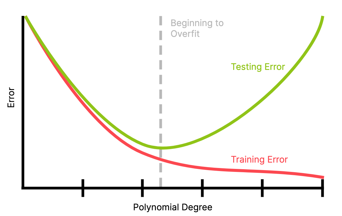
Chapter 9 - Generalization Errors and Evaluation of Models
A model's training error is the total cost of a model across all the training data.
As a model becomes more complex (e.g. the power of a polynomial regression gets higher), this can only go down, assuming the more complex parameter space is a superset of the old parameter space.
However, the training error only measures against training data; does it generalize to the data on which we actually want to use the model?
A model's generalization error is the expected cost of a model across all the possible datapoints, i.e. the whole data space. It measures how well a model is likely to perform on data it has never seen before.
Because the model has only been trained on its training data (by definition), it can only minimize cost over that training data. So, we can't train to minimize generalization error directly. What we can minimize is the empirical error.
Generalization error can be caused by overfitting, where the function has been overly adapted to the training data specifically; it matches the noise of the data instead of the trend. In the \(n\to\infty\) case, an overfitted function returns \(y_i\) if input \(x_i\) is in the dataset and \(0\) otherwise.
This is useless, because the whole reason we want to build a model is to predict data we haven't seen.
Overfitting happens when a model is too complex for its dataset.
A sign of overfitting is extremely large coefficients, since these can be used to target specific data points.
Underfitting can occur when the model is not complex enough to represent the data. However, this can be more easily detected, since both generalization and training error will remain high.
Test Sets
A test set is a subset of the dataset \(\mathcal{D}\) left out of training and used to test the model's performance; in particular to test for overfitting. Since the model hasn't seen the testing data before, it can't have overfit to it.
Aside: not being able to use all the data is a disadvantage of testing this way. Cross-validation can be used to split training data in such a way that we can get reasonable performance estimates for models trained on all the data.
Overfitting has likely occurred if the testing error is significantly higher than the training error, i.e. the generalization error is high.
Note: for a well-trained model, training error will likely be higher than testing error because, by definition, the model has seen the training data but not the testing data.
A good choice for a model is one that minimizes the training error, since this seems to generalize the best. Relative to this point, models with lower complexity likely underfit and and models with higher complexity likely overfit.
Underfitting has likely occurred if the next increase in complexity (e.g. additional power in polynomial regression) decreases both the training and testing error. As such, the "optimal" model is the one with the smallest testing error.
Making Statistical Claims about Error
Confidence Intervals
If we take the sample average of \(m\) error samples of function \(f\)'s estimation of dataset \(\mathcal{D}\), our sample average error is \(\overline{E}=\displaystyle \frac{1}{m} \sum\limits_{i=1}^{m}c_i(f)\), where \(c_i(f)\) is the error of sample \(i\) calculated by \(c\) (e.g. squared error, etc.). The sample average error follows a student's T distribution
The student's T distribution allows sample variance to be used instead of the true variance
So, \(\varepsilon=T[{\delta, m-1}] \displaystyle\frac{S_m}{\sqrt{m}}\) where \(S_{m}^{2}=\dfrac{1}{1-m}\displaystyle\sum\limits_{i=1}^{m}(c_i (f)-\overline{E})^2\) and the constant \(T[{\delta, m-1}]\) depends on the number of samples
Aside: this \(T\) table lookup is analogous for the \(Z\) table value of a gaussian distribution, but changes as a function of the number of samples \(m\) instead of remaining constant like \(Z[\delta]\) for a given \(\delta\). As \(m\to\infty\), \(T[{\delta, m}]\to Z[\delta]\), so the student's T distribution approaches the corresponding gaussian distribution
Confidence intervals effectively measuring the performance of one model, but also multiple. If for given \(\varepsilon_1\) and \(\varepsilon_2\), we have \(\overline{E_1}+\varepsilon_1 < \overline{E_2}-\varepsilon_2\) (i.e. the intervals don't overlap significantly*), we know that \(f_1\) is statistically significantly better than \(f_2\) with confidence level \(\delta\).
Parametric Tests
If we want to simply rank models \(f_1\) and \(f_2\) without precise error bars, we can perform a parametric test by testing a model on a dataset and calculating the probability that the result would happen randomly; this probability is called the \(p\)-value. Most consider that a \(p\) value of \(\alpha = 0.05\) or smaller implies statistical significance.
We are really considering whether it is more likely that the null hypothesis \(H_0\) (generally that the result happened randomly) is true, or whether the alternative hypothesis\(H_1\) is true, where \(H_1\) is the "positive hypothesis" (e.g. that a model predicts data). If \(p < 0.05\), we can reject the null hypothesis and accept \(H_1\).
Binomial Test
We can perform the binomial test between two models \(f_1\) and \(f_2\) by
For each point in the test set, record which model performs better. If the set has \(m\) points, \(f_1\) will "win" \(0\leq k \leq m\) times and and \(f_2\) will "win" \(m-k\) times.
\(H_0\) is the hypothesis that \(f_1\) and \(f_2\) have the same quality (i.e. that the result was due to random variance), and \(H_1\) is the hypothesis that \(f_1\) is better than \(f_2\) (assume WLOG that \(f_1\) performed better)
We define \(p=P(f_1 \text{ gets at least } k \text{ wins})=\displaystyle\sum\limits_{i=k}^{m}{m\choose i} \beta^{i}(1-\beta)^{m-i}\) from the PF of the binomial distribution, where \(\beta\) is the probability that \(f_1\) "wins" based on test set (likely around \(\frac{1}{2}\))
If \(p < 0.05\) (or more generally if \(p < \alpha\) for chosen \(\alpha\)), then we can reject \(H_0\) and state with statistical backing that \(f_1\) performs better
Other Tests
Although the structure of the testing is constant, different distributions can be used for different tests when necessary.
The test we choose depends on the distribution that our performance measure follows, i.e. the distribution arising from our tests
Each type of test makes assumptions about what kind of values we will find
E.g. if we considered the error of each \(f_1\) and \(f_2\) guess instead of just whether which one was the best, we would have two values in \(\mathbb{R}\) per trial; a paired t-test would be appropriate for this case.
Choosing a parametric test is like choosing a learning model: strong assumptions can lead to faster learning/stronger results, but are more prone to bias/poor prediction, whereas weaker models make better predictions but need more data
Often, we have less data available for statistical tests, making this decision even harder than choosing a model
Types of Errors
Type I error: A test is used under incorrect assumptions → the null hypothesis is rejected when it shouldn't have been (false positive)
Type II error: A test fails to reject the null hypothesis even though the data is statistically significant (false negative)
Can arise when the parametric test chosen is too weak (i.e. can be made stronger)
Chapter 10 - Regularization and Constraint of the Hypothesis Space
Note: Although motivating the actual regularization formulae, I didn't find the course notes explained this concept in a clear way, particularly when first introducing it. I would recommend reading this article on the subject first to provide some background before reading the course notes.
Regularization refers to a set of techniques used to reduce overfitting by trading training accuracy for generalizability. This is done by adding an additional term to the cost function that penalizes large coefficients in \(\vec{w}\), since this often indicates overfitting.
Deriving Regularization as MAP
If we define linear regressions as a MAP problem (instead of an MLE problem, like we have been), we must choose a prior\(p(\vec{w})\), since we are considering \(p( \vec{w}|\mathcal{D})\). This prior is picked to regularize overfitting. Two common choices are the Gaussian Prior (\(\ell_2\) norm) and the Laplace Prior (\(\ell_1\) norm).
It turns out that the implementation of regularization "pops out" of the equation when we consider linear regression as a MAP problem; it follows directly from this perspective!
In the following priors, \(\lambda\) is a hyperparameter (i.e. a parameter of the learning process itself). It ends up acting as the regularization parameter; the higher the \(\lambda\), the higher the penalty for having large coefficients.
Assume each component \(w_j\) of \(\vec{w}\) has Gaussian prior \(\mathcal{N}(0, \dfrac{\sigma^2}{\lambda})\) with the following assumptions
We assume that there is no covariance (and/or correlation) between weights
\(\lambda>0\) such that \(p(y| \vec{x}) = \mathcal{N}(\vec{x}^{\top}\vec{w},\sigma^2)\).
We choose \(\dfrac{\sigma^2}{\lambda}\) for the prior's variance in order to create a regularization parameter (namely \(\lambda\)).
Since each prior \(p(w_j)\) is gaussian, the prior \(p(\vec{w})\) is defined as \(p(\vec{w})=p(w_1)\times p(w_2)\times \dots \times p(w_d)\). Taking the log likelihood and expanding the gaussian probability function yields
The first term is constant, so it doesn't affect the selection of \(\vec{w}\).
Since we are using MAP, we consider the prior and the likelihood, so we want to find the \(\arg\min\) of their sum, so we get \[\arg\min\limits_{\vec{w}\in \mathbb{R}^{d+1}}-[\ln(p(\vec{y}|[\vec{X}, \vec{w}]))+\ln(p(\vec{w}))] = \dots = \arg\min\limits_{\vec{w}\in \mathbb{R}^{d+1}} \frac{1}{2}\sum\limits_{i=1}^{n}(\vec{x_i}^{\top}\vec{w} - y_i)^{2}\, + \frac{\lambda}{2}\sum\limits_{j=1}^{d}w^2_j\]
Since \(\vec{x_i}^{\top}\vec{w}\) is our prediction \(\hat{y_i}\), we simply have our regular MAP cost function plus the regularization term, here \(\displaystyle\frac{\lambda}{2}\sum\limits_{j=1}^{d}w^2_j\).
Since we have two terms in the cost function, the estimation now "balances" the objectives they both represent, respectively fitting the weights and not overfitting.
Note: the regularization terms doesn't include \(w_0\) since, as the intercept term, it only shifts the function
The gradient of our regularized cost function is \(\nabla c_i(\vec{w})=\begin{bmatrix}(\vec{x_i}^{\top}\vec{w}-y_i) \\ (\vec{x_i}^{\top}\vec{w}-y_i) x_{i1} + \lambda{w_1} \\ (\vec{x_i}^{\top}\vec{w}-y_i) x_{i2} + \lambda{w_2} \\ \dots \end{bmatrix}\)
We can simply the problem (and the PDF) by assuming the mean of each \(w_j\) is \(0\), assuming here we subtracted the intercept term \(w_0\) from it. So, we don't need to consider the \(w_0\) term either.
We define and motivate the Laplace prior in the same way as the Gaussian prior, but assume each component \(w_j\) of \(\vec{w}\) follows a Laplace distribution instead.
Performing the same derivation, we find the regularization term to be \(\displaystyle\frac{\lambda}{2}\sum\limits_{j=1}^{d}||w_j||\), the difference being that we no longer square \(w_j\). So, the Laplace prior is more likely to return terms where some \(w_j\) are \(0\).
Note: this objective is hard to optimize (e.g. with gradient descent) because the Laplace PDF is not differentiable at \(0\) (!). We will not optimize it in this course.
Expectation and Variance for MLE vs. MAP
In the (univariate) case where we have one parameter \(w\) (with "true" value \(\omega\)) over dataset \(\mathcal{D}=(X,Y)\), we have found in [[Chapter 5 - Parameter Estimation]] that the MLE estimation \(w_{\text{MLE}}(\mathcal{D})=\dfrac{\sum_{i=1}^{n}X_i Y_i}{\sum_{i=1}^{n}X_i^2}\) is an unbiased estimator of \(\omega\); we can find variance using the formula (in the course notes on [[CMPUT 267 Notes.pdf|page 107]]).
We can derive the variance for \(w_{\text{MLE}}\) as \(\text{Var}[w_{\text{MLE}}]=\sigma^{2}\mathbb{E}\left[ \dfrac{1}{n} C^{-1}_n \right]\) where \(C_n := \displaystyle \frac{1}{n}\sum\limits_{i=1}^{n}X^{2}_i\)
So, for very small amounts of data, \(C^{-1}_n\) can be very large, and thus \(w_{\text{MLE}}\) can vary widely
\(w_{\text{MLE}}\) being very different on small subsets of the same dataset is not desirable!
However, the MAP estimate \(w_{\text{MAP}}(\mathcal{D})=\dfrac{\sum_{i=1}^{n}X_i Y_i}{\lambda+S_n}\) is not an unbiased estimate of \(\omega\); we find that \(\displaystyle\mathbb{E}[w_{\text{MAP}}(\mathcal{D})]=\omega \mathbb{E}\left[\frac{S_n}{\lambda+S-n}\right]\). So, it is unbiased when \(\lambda=0\) and as \(\lambda\to 0\) (i.e. when the regularization penalty is \(0\), as expected), but becomes more biased as \(\lambda\to \infty\)
Once again, we can derive the variance. We find \(\text{Var}[w_\text{MAP}]=\sigma^{2}\mathbb{E}\left[\displaystyle \frac{1}{n} C^{-1}_{n, \lambda} C_n C^{-1}_{n, \lambda} \right]\) where \(C_{n, \lambda} = \dfrac{1}{n}(\lambda+ S_n)\)
Notice than when \(C_n\) (essentially sample estimate for variance of \(X_i\)) is small, \(\text{Var}[w_\text{MAP}]\) doesn't get large like \(\text{Var}[w_\text{MLE}]\) since \(C^{-1}_{n, \lambda} < \dfrac{1}{\lambda}\). So, as \(\lambda\to \infty\), \(\text{Var}[w_\text{MAP}]\) gets arbitrarily small.
Bias-Variance Tradeoff Revisited
We find that we can reduce the mean-squared error by incurring some bias; this is optimal as long as the variance is decreased more than the squared bias increases.
Remember, we are assuming the underlying function is indeed linear, and thus that all the bias is introduced by regularization. In reality, bias can also come from choosing a function class that can't truly estimate the underlying function (e.g. trying to predict a cubic function with a linear regression).
Bias-Variance Quadrants
Low bias, low variance: \(\mathcal{F}\) is large enough (i.e. has enough "detail") to represent \(\star{f}\) properly. The more complex \(\star{f}\) is, the more samples are required
Low bias, high variance: \(\mathcal{F}\) is complex enough to represent \(\star{f}\), but we don't have enough samples (\(n\) is too small)
High bias, low variance: \(\mathcal{F}\) is not complex enough to represent \(\star{f}\)
High bias, high variance: Bad Bad Bad. Likely not enough data and the model \(\mathcal{F}\) is not complex enough to represent \(\star{f}\).
Choosing the Right Model
Bias-variance Tradeoff (again)
Generally, we find above that the smaller our dataset is, we should err on the side of simpler models so that we don't end up in the useless high-bias, high-variance category.
We can use a small validation set as data to train a bunch of different models, then evaluate which model would perform the best with the full testing set.
This is used to appropriately constrain which models we consider
The validation set is often split off of the training set
Inductive Bias
We can use inductive biases to improve models: these are biases that we are aware of (from our prior knowledge) that we can use to prune the function space.
In theory, a good enough model with enough data could learn the same things we know already. However, it can be helpful to manually nudge the model in the right direction with prior knowledge
We are manually biasing the model
E.g. in an image dataset, we know that the red channel contains no useful data. In theory, the model could learn this by itself with the right data, but we can simply write the model to ignore the red data immediately to increase accuracy.
However, this starts to nudge ML models from things that should be able to learn from any context (i.e. from any dataset) to things more tailored to situations useful to us.
Manually biasing a model might reflect the biases we hold; shouldn't machine learning be a tool to get an unbiased preception of data?
E.g. large language models should be general enough to "understand" any language. However, it is most "useful" (profitable) to optimize the models to learn english. We can introduce biases to help this (i.e. hard-coding some grammar rules), but this makes the model worse at understanding other languages.
Chapter 11 - Logistic Regression and Linear Classifiers
Logistic regression lets us apply the machinery of regression to classification problems by interpreting the parameterization of the estimated logistic regression as a classification
We learned that classification requires estimating \(p(y|\vec{x})\). For binary classification, i.e. \(\mathcal{Y}=\set{0, 1}\), \(p(y|\vec{x})\) must follow a Bernoulli distribution, which has one parameter \(\alpha\); \(\alpha(\vec{x})=p(y=1|\vec{x})\). We can use logistic regression to parametrize and learn this \(\alpha(\vec{x})\).
Parametrization for Binary Classification
Essentially, we perform linear regression, but constrain the range of the function to \([0, 1]\), since this is the space over which binary classification is (somewhat) defined. We constrain using the sigmoid function\(\sigma : \mathbb{R}\to (0, 1), w \mapsto (1+\exp{w})^{-1}\); we aim to learn weights \(\vec{w}\) such that \(p(y=1|\vec{x})=\sigma(\vec{x}^{\top}\vec{w})\)
We find \(p(y|\vec{x})=\sigma(\vec{x}^{\top}\vec{w})^{y}(1-\sigma(\vec{x}^{\top}\vec{w}))^{y-1}\)
So, our prediction function is in the form \(f(\vec{x})=\sigma(\vec{x}^{\top}\vec{w})\) for weights\(\vec{w}\).
This uses the same approach as polynomial regression
Since this prediction is in \((0, 1)\), not \(\set{0, 1}\), we must convert \((0, 1)\to\set{0, 1}\). Generally, if \(f(\vec{x})>0.5\), it is classified as \(1\), otherwise \(0\). So, the function we are using is \(\text{round}\).
Any "rounding point" value can be used, \(0.5\) is the most common. This is related to "unbalanced cost functions"; sometimes a false negative is worse than a false positive.
Aside: how can this be formally defined in terms of a cost function?
The distribution of the actual probabilities is still useful; if most of \(f\)'s values are above \(0.9\) or below \(0.1\), the model is more confident than if most values hover around \(0.5\), even if the "cutoff point" is the same.
\(f\)actually gives a confidence value for \(\vec{x}\) being classified as \(1\); the conversion step to \(\set{0, 1}\) is only needed to act on that information.
MLE For Logistic Regression
Like in any MLE estimation, we choose \(f\) to maximize \(p(\mathcal{D}|f)\) for dataset \(\mathcal{D}\), so our objective (also called cross-entropy) \(c(\vec{w})\) is \(c(\vec{w}) = \dfrac{1}{n} \displaystyle\sum\limits_{i=1}^{n}-\ln{p(y_i | \vec{x_i})}\). We find that the gradient (for a single entry in \(\vec{w}\)) is \(\nabla c(w_i) = (p_i-y_i)x_{ij}\), where \(p_i=\sigma((\vec{x}^{\top}\vec{w})_i)\)
\(\nabla c(\vec{w})=0\) doesn't have a closed form solution, so we must use an iterative optimization method like gradient descent.
The stochastic gradient descent rule for \(b=1\) is (trivially) \(\vec{w_{t+1}}=\vec{w_t}-\eta_t (\sigma(\vec{x_i}^{\top}\vec{w_t})-y_i)\vec{x_i}\)
We can also incorporate a Gaussian or Laplace prior to derive a regularized version: for a Gaussian prior (\(\ell_2\) regularization), we find the gradient descent rule \(\vec{w_{t+1}}=\vec{w_t}-\eta_t (\sigma(\vec{x_i}^{\top}\vec{w_t})-y_i)\vec{x_i} - \eta_{t}\dfrac{\lambda}{n}\vec{w}_t\)
Logistic Regression for Linear Classification
Because \(\vec{x}^{\top}\vec{w}=0\) represents a hyperplane that splits \(\mathbb{R}^n\) into two regions, it is a linear classifier (even though \(\vec{w}\) was learned with the non-linear \(\sigma\)).
The intercept term \(w_0\) of this plane prevents the result from being biased by preventing it from being skewed towards the origin. If the term were not present, the hyperplane would have to pass through the origin.
By definition, any \(\vec{x}\) satisfying this is orthogonal to \(\vec{w}\)
Aside: this is what classifiers do: partition space \(\mathbb{R}^n\) into equivalence classes. If a classifier is linear, this boundary is shaped like a hyperplane, but it can (and often should) be shaped differently.
Issues with Minimizing MLE
Why didn't we directly try to minimize \(c(\vec{w}) = \dfrac{1}{n} \displaystyle\sum\limits_{i=1}^{n}(\sigma(\vec{x_i}^{\top}\vec{w})-y_i)^2\) (or the equivalent with a different cost function) instead of this Bernoulli skedaddling? Because this is non-convex optimization.
Specifically, for the squared error (euclidean error), there are exponentially many local minima
Chapter 12 - Bayesian Linear Regression
In the previous chapters, we used point estimates MLE and MAP to characterize linear regression. In this chapter, we use Bayesian estimation to do the same, namely Bayesian estimation of the conditional distribution \(p(y|\vec{x})\).
Like before, using Bayesian estimation gives us credible ranges around our predictions, this time weights for the linear model.
The following derivations consider the univariate case with one weight \(w\) for simplicity.
Posterior Distribution \(p(w|\mathcal{D})\) for Known Noise Variance
Once again, we make the assumption that \(p(y|x)\sim \mathcal{N}(\mu=xw,\sigma^2)\) and that each component (weight) \(w_i\) has a gaussian prior \(p(w_i)\sim \mathcal{N}(0, \dfrac{\sigma^{2}}{\lambda})\) (we take the prior \(p(w)\) to be conjugate to the posterior \(p(\mathcal{D}|w)\), i.e. Gaussian in this case). From Bayes rule, \(p(w|\mathcal{D})=\dfrac{p(\mathcal{D}|w)p(w)}{p(\mathcal{D})}=\displaystyle \frac{p(w)\prod_{i=1}^{n}p(y_i|x_i, w)}{\int p(w)\prod_{i=1}^{n}p(y_i|x_i, w) \, dw}\).
Note: we use the same prior as in \(\ell_2\) regularization
We can derive that \(p(w|\mathcal{D})\sim \mathcal{N}(\mu_n, \sigma^2_n)\) where \(\sigma^2_n=\dfrac{\sigma^2}{\sum_{i=1}^{n}x_i^{2}+\lambda}\) and \(\mu_n=\dfrac{\sum_{i=1}^{n}x_i y_i +\lambda\mu _0}{\sum_{i=1}^{n}x_i^2+\lambda}\).
The MAP solution corresponds to the mode \(\mu_n\) of this distribution
Since this is a Bayesian estimation, we can establish a credible interval with \(\sigma^2_n\), since this term gets smaller as \(n\to \infty\). Namely, for a \(\delta\) credible interval, we compute \(p(w\in [a, b]|\mathcal{D})=\delta\)
Since we chose a Gaussian prior \(p(w)\), we can simply pick \(a=\mu_n -Z[\delta]\sigma_n, b=\mu_n +Z[\delta]\sigma_n\) using the Gaussian z-table
This is different than (although very similar to) a confidence interval because the prior is used to calculate the interval in addition to the data (\(\mathcal{D}\)) itself
Posterior Distribution \(p(w|\mathcal{D})\) for Unknown Noise Variance
Generally, we don't know the variance \(\sigma^2\) when taking a linear regression since we don't understand the data's noise before analyzing the data itself.
In this case, the conjugate prior follows the Normal-Inverse-Gamma distribution, which has parameters \(\mu_n, \lambda_n, a_n, b_n\)
If the parameters of our prior's distribution are \(\mu_0\in \mathbb{R}\) and \(\lambda_0, a_0, b_0 > 0\), we find that the posterior (and variance) \(p([w, \sigma^2]|\mathcal{D})=\text{NIG}(\mu_n, \lambda_n, a_n, b_n)\), where \(\lambda=\displaystyle\sum\limits_{i=1}^{n}x^2_i+\lambda_0\), \(\mu_n=\dfrac{\sum_{i=1}^{n}x_i y_i+\lambda_0 \mu_0}{\lambda_n}\), \(a_n=a_0+\frac{1}{2}n\), \(b_n=b_0+ \dfrac{1}{2}\left(\displaystyle\sum\limits_{i=1}^{n}y^{2}_i+\lambda_0\mu_{0}^{2}-\lambda_n\mu_n^2\right)\)
The mode of a NIG distribution is \(\mathbb{E}[(w, \sigma^2)]=(\mu_n, \frac{b_n}{{a_n -1}})\). So, \(\dfrac{b_n}{{a_n -1}}\) is the most likely value for the variance \(\sigma^2\) of the noise
The course notes contain a derivation of a variance equation for a simpler set of parameters to the NIG distribution
Under NIG, the variance on the choice for the weight \(w\) is given by \(\dfrac{b_n}{{(a_n -1)}\lambda_n}\)
If this term is large, the credible interval around our choice of weight is also large
The marginal distribution of \(w\) for NIG is a Student's t distribution, so we can calculate confidence intervals for confidence \(\delta\) with \([\mu_n-\varepsilon, \mu_n+\varepsilon]\) where \(\varepsilon=\dfrac{a_n}{b_n \lambda_n}T[{1-\delta,2a_n}]\)
The Posterior Predictive Distribution
Why go to the trouble of using Bayesian Linear Regression?
It is more useful to reason about the variability across our predictions using \(w\), rather than the variability of \(w\) itself under a particular distribution. Specifically, we want to know \(P(xw|[x, \mathcal{D}])\)
This is still a student's T distribution (since the \(x\) isn't really changing anything here), so an interval of confidence \(\delta\) is given by \([x\mu_n-\varepsilon, x\mu_n+\varepsilon]\) where \(\varepsilon=\dfrac{a_n}{b_n \lambda_n}T[{1-\delta,2a_n}]\).
If error is known, the distribution is Gaussian with mean \(x\mu_n\) and variance \(x^{2}\sigma^2_n\)
The Posterior predictive distribution\(p(y|x,\mathcal{D}\displaystyle)=\int_{w}p(w|D)p(y|[x, w])\, dw\) is method of model averaging that weights each model (value of \(w\)) proportionally to how effective it is.
Since we are using Bayesian linear regression, we know the closed form of all the distributions in the equation, so we can evaluate the integral analytically!
For known variance, we find \(p(y|[x, \mathcal{D}]) \sim \mathcal{N}(x\mu_n,x^2\sigma^2_n+\sigma^2)\)
Things are more complicated when noise is unknown, but it still follows a student's T distribution