Chapter 1 - Introduction - Symmetries in the Plane
If algebra is the study of structure, then group theory is the study of symmetry.
Symmetries from Geometry
A canonical example for introducing groups is the symmetries of regular polygons (we will see later that these correspond to the dihedral groups\(D_n\)). Polygons may be symmetric with respect to rotation and/or reflection; "applying" two symmetries to a shape will yield another symmetry. This is the structure of a group.
We can represent a group's structure with a multiplication table that contains the result of "operating" on any two elements. By convention, the column indices of the table corresponds to the first operand and the row indices correspond to the second operand.
This matters because commutativity isn't given: we may have \(a \circ r \ne r \circ a\);
Every element in the set of symmetries must appear exactly once in each row and column (we will prove why later, as an assignment question).
Note that symmetries of a square can be seen as functions in \(\mathbb{R}^{2}\) that map the square back to itself. This is an important idea.
For reflections, we need an extra dimension; a reflection in \(\mathbb{R}^2\) can be "executed" as a rotation in \(\mathbb{R}^3\) that "flips" \(\mathbb{R}^2\).
The platonic solids are also good examples for finding symmetries.
Symmetries of the Roots of a Polynomial in \(\mathbb{R}[X]\)
Theorem 1.1: Fundamental Theorem of Algebra
Theorem
A polynomial \(f(X)\in \mathbb{R}[X]\) of degree \(n\) must have \(n\) roots (with multiplicity) in \(\mathbb{C}\).
If \(a+bi\in \mathbb{C}\) is a root of \(f(X)\), then its conjugate\(a-bi\) must also be a root of \(f(X)\) as well.
Here, conjugates provide a symmetry that is "like" a reflection with respect to the real axis.
We also see symmetry in roots of unity, i.e. the roots over \(\mathbb{C}\) of the equation \(f(X)=X^{k}-1\) for fixed \(k\in \mathbb{N}\). In closed form, these roots are \(\displaystyle \cos{\frac{2 \pi n}{k}} + i\sin{\frac{2 \pi n}{k}} =: e^{\frac{2 \pi i n}{k}}\) for \(n\in \set{1, 2, \dots, k}\), which describe the vertices of a regular \(k\)-gon centered at \((0,0)\) with "radius" \(1\) on the complex plane. These roots form a group under multiplication.
Permuting roots of polynomials leads into Galois theory.
Symmetries and Isometries of \(\mathbb{R}^n\)
Definition 1.2A: Linear Isometry in \(\mathbb{R}^n\)
Definition
A linear isometry\(T\) in \(\mathbb{R}^n\) is a linear transformation \(T : \mathbb{R}^{n}\to \mathbb{R}^{n}\) such that \(\| T(\vec{u}) - T(\vec{v}) \|=\| \vec{u}-\vec{v} \|\).
So, by definition, any two points \(\mathbb{R}^3\) stay the same "distance" away from each other after being transformed by a linear isometry.
Alternate characterization: the matrix representing a linear isometry has determinant \(1\) or \(-1\). If the determinant is \(1\), no "flip" has occurred; such an isometry is called a rigid transformation.
We can prove this preserves angle as well; thus linear isometries preserve inner products.
We can generalize linear isometry to metric spaces by defining in terms of an arbitrary distance function instead of the Euclidean norm:
Definition 1.2B: Isometry in a Metric Space
Definition
An isometry is a map \(T : X \to Y\) between metric spaces\(X, Y\) that preserves distance, i.e. such that for all \(a, b \in X\), we have \(d_X(a, b)=d_Y(T(a), T(b))\).
Definition 1.2C: Affine Isometry in \(\mathbb{R}^n\)
Definition
An affine isometry\(\tau\) in \(\mathbb{R}^n\) is a linear transformation \(\tau : \mathbb{R}^{n}\to \mathbb{R}^{n}\) of the form \(\tau(\vec{u}):=T(\vec{u})+\vec{b}\) where \(T:\mathbb{R}^{n}\to \mathbb{R}^n\) is a linear isometry and \(\vec{b}\in \mathbb{R}^n\) is fixed. In the context of linear algebra, we may also call this an affine transformation.
We can characterize an affine isometry is a linear isometry (\(T\) in the definition) and a translation by \(\vec{b}\).
Definition 1.3: Symmetry in \(\mathbb{R}^n\)
Definition
A symmetry\(S\) in \(\mathbb{R}^n\) of geometric object \(P\) is a function \(f: \mathbb{R}^{n}\to \mathbb{R}^n\) that preserves the distance between any two points in \(P\).
Proposition 1.4
Proposition
Let \(P\) be a polytope in \(\mathbb{R}^n\) with its centroid (center of mass) at \(\vec{0}\). Any symmetry of \(P\) must be a linear isometry of \(\mathbb{R}^n\).
Finally, we note (as a well-known linear algebra result) that the composition of linear transformations corresponds to the multiplication of the corresponding matrices of the transformations. So, any relationship that exists between multiple transformations also exists between the matrices.
This is because there is a trivial homomorphism between the set of invertible transformations under composition and the group of invertible matrices under multiplication
Chapter 2 - Modular Arithmetic
Oops! All number theory.
For \(a, n \in \mathbb{Z}\) with \(n\ne 0\), we can always find \(q, r\in \mathbb{Z}\) and \(0\leq r \leq |n|\) such that \(\boxed{a=qn+r}\), i.e. we can divide any two numbers if we allow for a non-zero remainder. This is Euclidean division.
The size of the remainder\(r\) is bounded by \(|n|\).
If \(r=0\), we say \(n\)divides\(a\), written \(n \mid a\).
Theorem 2.1: Bézout's Lemma
Theorem
For any nonzero \(a, b\in \mathbb{Z}\), there exist \(x, y \in \mathbb{Z}\) such that \(ax+by=\text{GCD}(a, b)\)
For integers \(a, b\) and nonzero natural number \(n\), we say "\(a\) is congruent to \(b\) modulo \(n\)" (denoted \(a \equiv b \mod n\)) iff \(n\) divides \(a-b\).
If two numbers are congruent mod \(n\), they yield the same remainder when divided by \(n\)
Congruence mod \(n\) is an equivalence relation, so we can partition \(\mathbb{Z}\) into equivalence classes. These ones in particular are called congruence classes and are denoted \([a]_n :=\set{b\in \mathbb{Z} \mid a\equiv b \mod n}=\set{a+kn \mid k\in \mathbb{Z}}\) (the \(n\) is generally omitted, and often left as a free variable anyway).
E.g. \([5]_3 = [2]_3\) since \(5\) and \(2\) both have remainder \(2\) when divided by \(3\).
We define \(\mathbb{Z}_n\) as the set of congruence classes mod\(n\), i.e. \(\mathbb{Z}_n := \set{[a] \subseteq \mathbb{Z} \mid a \in \mathbb{Z}}\); any element in \([a]\) can represent its congruence class.
By the bound on the remainder, each remainder has exactly one class, and each class corresponds to a remainder. So, \(\mathbb{Z}_n\) has \(n\) elements, namely \(\set{[0], [1], \dots, [n-1]}\).
Addition and multiplication are well-defined with respect to congruence classes, i.e. for any choices of representatives, the corresponding representative given by the operation will be in the correct congruence class. Symbolically, \([a]+[b]=[a+b]\) and \([a]\cdot [b]=[a\cdot b]\).
This notion of well-definedness comes up later when considering cosets.
Chapter 3 - Group Definitions and Examples
Its time
Definition 3.1: Group
Definition
A group\((G, \,\square\, )\) consists of a set \(G\) of elements and a binary operation\(\,\square\, : G \times G \to G\) which adhere to the following group axioms:
Associativity: \(a \,\square\, (b \,\square\, c) = (a \,\square\, b) \,\square\, c\) for all \(a, b, c \in G\).
Identity/Neutral Element: There exists some \(e \in G\) such that \(e \,\square\, a = a \,\square\, e = a\) for all \(a \in G\)
Inverses: Each element \(a \in G\) has an inverse\(a^{-1}\) such that \(a \,\square\, a^{-1} =a^{-1} \,\square\, a = e\)
E.g. \((\mathbb{Z}, +)\), \((\mathbb{Q}, +)\), \((\mathbb{R}, +)\), and \((\mathbb{C}, +)\) are all groups
E.g. \((\mathbb{R}^{\times}, \cdot)\) is a group, where \(\mathbb{R}^{\times}:= \mathbb{R}\setminus\set{0}\), since \(0\) does not have a multiplicative inverse in \(\mathbb{R}\). \(\mathbb{Q}^\times\) and \(\mathbb{C}^\times\) also form groups under multiplication, but \(\mathbb{Z}^\times\) does not because only \(1, -1\) have multiplicative inverses.
E.g. any ring \((R, \oplus, \odot)\) implies a group \((R, \oplus)\)
\((\mathbb{Z}_n \setminus\set{[0]}, \cdot)\) is a group if and only if \(n\) is a prime number. If \(n\) is composite, \(\mathbb{Z}_n\) will have zero-divisors (e.g. \([a], [b]\) such that \([a]\cdot [b] = [n]=[0]\)), contradicting closure.
In particular, it is useful to characterize known structures from linear algebra in terms of groups:
The set \(M_{m\times n}(\mathbb{F})\) of \(m\times n\) matrices over a field \(\mathbb{F}\) is a group under addition, but not matrix multiplication. However, the general linear group\(\text{GL}_n(\mathbb{F}):\set{A \in M_n(\mathbb{F}) \mid \det{A} \ne 0}\) of invertible\(n\times n\) matrices does form a group under matrix multiplication.
In this course, we choose \(\mathbb{R}\) for our field, i.e. we speak of \(\text{GL}_n(\mathbb{R})\).
More generally, the set of linear transformations \(\text{GL}(V) := \set{T : V \to V \mid T \text{ is linear and invertible }}\) forms a group under composition. We note that this is the "same" group as \(\text{GL}_n(\mathbb{F})\) iff \(\dim_{\mathbb{F}}{V}=n\).
The orthogonal group\(O_n(\mathbb{F}) := \set{A \in M_n(\mathbb{F}) \mid AA^{\top}= I_n = A^{\top}A}\) is a group under matrix multiplication; inverses are given by \(A^{-1}=A^\top\).
If \(T : \vec{u}\mapsto A \vec{u}\) is a linear isometry, then \(A\in O_n(\mathbb{F})\) is in the orthogonal group
So, matrices in the orthogonal group represent transformations under which the inner product is invariant, i.e. orthogonal transformations preserve distances and angles.
In \(\mathbb{R}^2\), these are the distance-preserving transformations with a fixed point.
Definition 3.3: Invertible Congruence Classes
Definition
\(\Phi(n)\) denotes the set of congruences classes \([a]\in \mathbb{Z}_n\) that are invertible in \(\mathbb{Z}_n\). So, we have \(\Phi(n)\subseteq \mathbb{Z}_n\).
Theorem 3.4: \(\Phi(n)\) is a Group
Theorem
We have \(\Phi(n) := \set{[a]\in \mathbb{Z}_n \mid \text{GCD}(a, n)=1}\), i.e. \(\Phi(n)\) is the set congruence classes \([a]\) whose representatives \(a\) share no factor with \(n\).
\(\Phi(n)\) is a group under \(\mathbb{Z}_n\)'s multiplication.
Proof sketch (1): invertible → \([a][x]=[1]\) → \(ax\equiv 1 \mod n\) → \(ax-1=ny\) for some \(y\). If some common factor \(d\) divides both \(a\) and \(n\), then it divides \(ax-ny\) by Bézout's lemma; thus \(d\mid 1\) and thus \(d\) is \(1\) or \(-1\), so \(\text{GCD}(a, n)=1\). We can essentially perform this derivation in reverse to show the other direction
We can prove (2) by simply checking the group axioms
We can find the inverse \([a^{-1}]\) of \([a]\) in \(\mathbb{Z}_n\) by using the Euclidean algorithm to \(a\) and \(n\) until we find remainder \(1\). Then, we re-write \(r_n = r_{n-1} \cdot k + 1\) as \(1 = r_n - r_{n-1}\cdot k\), then continue expanding everything out in reverse from how we found it with the Euclidean algorithm.
Note: in further math, many of the most interesting and useful group are under composition (\(\circ\)). This is a little more abstract since it acts on functions/transformations/etc. instead of "values".
Chapter 4 - Permutations
Definition 4.1: Permutation
Definition
A permutation\(\pi\) of \(X\) is a bijective function \(\pi : X \to X\).
This makes sense after first learning it; of course a bijective function "re-orders" its domain. And of course a permutation must be injective and surjective by definition.
It is common to represent permutations as \(\pi = \begin{bmatrix}1 & 2 & 3 & \dots & n \\ \pi(1) & \pi(2) & \pi(3) & \dots & \pi(n) \end{bmatrix}\).
Since permutations are bijective, we can combine them with composition, i.e. by performing one after the other. We have \(\pi_1 \circ \pi_2 = \begin{bmatrix} 1 & 2 & 3 & \dots & n \\ \pi_1 (\pi_2(1)) & \pi_1 (\pi_2(2)) & \pi_1 (\pi_2(3)) & \dots & \pi_1 (\pi_2(n)) \end{bmatrix}\)
Definition 4.2: \(\text{Sym}(X)\)
Definition
We define \(\text{Sym}(X)\) as the set of all permutations of the set \(X\). So, \(\text{Sym}(X)\) is a set of functions. We define the symmetric group\(S_n\) as the set of permutations of the set \(\set{1, \dots, n}\) specifically; \(S_n := \text{Sym}(\set{1, \dots, n})\).
Proposition 4.3: \(\text{Sym}(X)\) is a Group
Proposition
Let \(X\) be a set. Then, the set \(\text{Sym}(X)\) of all permutations of \(X\) is a group under composition \(\circ\).
Proof: A composition of two permutations \(\pi_1, \pi_2\) of \(X\) is another function mapping \(X\to X\) because both \(\pi_1\) and \(\pi_2\) are bijections. From here, checking the proposition against the group axioms is trivial.
The identity element of \(\text{Sym}(X)\) is the permutation \(\begin{bmatrix} 1&2&3&\dots \\ 1&2&3&\dots \end{bmatrix}\) and the inverse element is the permutation of \(\text{Sym}(X)\) is \(\pi ^{-1}=\begin{bmatrix} \pi(1)&\pi(2)&\pi(3)&\dots \\ 1&2&3&\dots \end{bmatrix}\).
In particular, we can find the inverse permutation by switching the rows of the \(n\times 2\) matrix representation (then reordering the columns to sort by the first element)
If \(\pi\) is a transposition, \(\pi^{-1}=\pi\) since we simply "swap back"; thus transpositions are involutions.
A cyclic permutation or cycle is a permutation of the form \(i_1 \mapsto i_2 \mapsto i_3 \mapsto \dots \mapsto i_k \mapsto i_1\), i.e. where each element in the cycle is "shifted" to the right, e.g. \(\begin{bmatrix} 1&2&3&\dots&k \\ 2&3&4&\dots &1 \end{bmatrix}\).
We may notate the cycle above as \((2, 3, 4, \dots, 1)\)
The order of this sequence matters; \((1, 2, 3)\) gets shifted differently than \((1, 3, 2)\).
Note: a subset of a permutation may be a cycle, e.g. \((2, 5, 4, 8)\) corresponds to the permutation \(\begin{bmatrix} 1&2&3&4&5&6&7&8 \\ 1&5&3&8&4&6&7&2 \end{bmatrix}\). The unchanging elements in this permutation are fixed.
Graphically, we can convert cycle notation to two-row notation by writing the cycle, then writing the cycle again below it, but shifted one element to the left.
Two cycles are disjoint if they cycle disjoint sets of elements.
Disjoint cycles are commutative: applying both yields the same result, no matter the order.
Theorem 4.4: Cycle Decomposition Theorem
Theorem
Every permutation \(\pi\) of a finite set \(X\) can be expressed as a product as disjoint cycles \(\pi_1, \dots, \pi_k\), i.e. \(\pi=\pi_k \circ \pi_{k-1} \circ \dots \circ \pi_2 \circ \pi_1\). This decomposition is unique up to the "starting point" of each cycle.
The proof of the Cycle Decomposition theorem follows structurally from the algorithm below; it uses induction on \(|X|\).
Algorithm for finding Cycles in a Permutation
Algorithm
Check which elements are fixed in the overall permutation \(\pi\); these are cycles of length \(1\) and will be as-is in the product.
Consider an element in \(X\) (e.g. \(1\)) and follow where it gets sent when it is repeatedly permuted; i.e. the sequence \(1, \pi (1), \pi(\pi(1)), \dots\). Clearly, this will eventually come back to \(1\) (see aside below) because \(X\) (and thus \(\text{Sym}(X)\)) is finite. This reveals a cycle.
Find the first element not in the cycle and repeat this process.
Eventually, each element will be in a cycle.
Aside: the structure of permutation groups lend themselves to graph-theoretic arguments: a permutation \(\pi\) is shaped like a directed graph where \(V(G)=X\) and an arc from \(a\) to \(b\) exists iff \(\pi\) sends \(a\mapsto b\). The resulting graph's vertices all have in-degree and out-degree \(1\). For example, the proof of the Cycle Decomposition Theorem follows naturally from thinking in terms of components and Eulerian paths.
The inverse of a permutation will retain the structure of the cycle decomposition, but reverse the direction of each cycle. Fixed points and transpositions will remain unchanged because they are involutions.
Permutations \(\pi_1, \pi_2\) are conjugate if there exists a third permutation \(\sigma\) such that \(\pi_1 = \sigma\circ \pi _2 \circ \sigma^{-1}\).
Theorem 4.6: Same Cycle Structure \(\iff\) Conjugate
Theorem
Permutations \(\pi_1, \pi_2\) are conjugate if and only if they have the same number of cycles of each length.
Aside: it will seem like the "cycle sequence" generating series \(\phi : \mathbb{N}\to \mathbb{N}\) describing how many cycle of each length a permutation has is invariant under isomorphism.
Proof sketch \(\implies\): we assume \(\pi_1 = \sigma\circ \pi_2 \circ \sigma\). We can break \(\pi_2\) down into its cycles and insert pairs, \(\sigma^{-1}\), \(\sigma\) between each cycle in the composition; these cancel out to \(\text{id}\), so they don't change the value. By associativity, each cycle in \(\pi_2\) gets transformed into \((\sigma \circ \pi_{2,i}\circ \sigma)\); so, each cycle in \(\pi_2\) has a corresponding (conjugate) cycle in \(\pi_1\). Thus, \(\pi_1\) and \(\pi_2\) have the same "cycle sequence".
Proof sketch \(\impliedby\): We pick a permutation \(\sigma\) that preserves cycles, i.e. that doesn't map two elements in a cycle to different cycles. Thus, the conjugation maps the old cycles to the new cycles, permutes those, then (inversely) maps the permuted new cycles back to the old ones, assuring conjugacy.
Note: the full proof has a few points of interest:
\(\text{id}\) trick: in a group theory proof, we can replace \(\text{id}\) with some \(\sigma\circ\sigma^{-1}\) or \(\sigma^{-1}\circ\sigma\) and continue deriving from there
In \(\implies\), we have a long chain of \((\sigma\circ \pi_1\circ \sigma^{-1})\circ(\sigma\circ \pi_2\circ \sigma^{-1})\circ\dots\), which by associativity cancels to \(\sigma\circ\pi_1\circ(\sigma^{-1}\circ\sigma)\circ\pi_2\circ(\sigma^{-1}\circ \sigma)\circ\dots\), which cancels to \(\sigma\circ \pi_1 \circ \dots \circ \pi_k \circ \sigma^{-1}\). This kind of cancellation structure is useful
E.g. diagonalization of matrices
E.g. telescoping series
Lemma 4.7: Conjugate of a cycle
Lemma
If \(\sigma \in S_n\) and cycle \(\pi = (a_1, a_2, \dots) \in S_n\), we have \({\sigma \circ \pi \circ \sigma^{-1}=(\sigma(a_1), \sigma(a_2), \dots, \sigma(a_k))}\)
I.e. the conjugate of a cycle is a permutation of the elements of that cycle
Proof: clearly \({\sigma \circ \pi \circ \sigma^{-1}}\) permutes \(\set{1, 2, \dots n}\); we just need to derive what this permutation is. We define \(\rho := (\sigma(a_1), \sigma(a_2), \dots \sigma(a_n))\); note that proving \({\sigma \circ \pi \circ \sigma^{-1}}=\rho\) is equivalent to proving \(\rho \circ \sigma(a_i)=\sigma \circ \pi(a_i)\). We have \(\rho \circ \sigma(a_i)=\rho(\sigma(a_i))=\sigma(a_{i+1})\) and \(\sigma\circ \pi(a_i)=\sigma(\pi(a_i))=\sigma(a_{i+1})\), so these two are equal for all \(a_i\). For \(b\ne a_i\) for all \(i\), \(b\) is not in the cycle → \(b\) is fixed by \(\pi\) → \(\sigma(b)\ne \sigma(a_i)\) since \(\sigma\) is injective → \(b\) is fixed by \(\rho\); it follows that \(\sigma\circ \pi(b)=\rho\circ \sigma(b)\)
If we have cycles \(\pi_1 = (a_1, a_2, \dots, a_n)\) and \(\pi_2=(b_1, b_2, \dots, b_n)\), then we can pick permutation \(\sigma\) such that \(\sigma\circ \pi_2 \circ \sigma^{-1}=\pi_1\) by defining \(\sigma(b_i):= a_i\).
So, given non-cycles \(\pi_1\) and \(\pi_2\), we can find \(\sigma\) such that \(\sigma\circ \pi_2 \circ \sigma^{-1}=\pi_1\) by decomposing \(\pi_1\) and \(\pi_2\) into cycles (they must have the same structure since they conjugate), using the formula above to convert the cycles, then converting back with \(\sigma^{-1}\).
Such a \(\sigma\) isn't unique: if \(\pi_1, \pi_2\) have "cycle generating sequence" \(\displaystyle\sum\limits_{k=0}^{\infty}a_k x^k\), then there are \(\displaystyle\frac{n!}{\displaystyle\prod_{k=0}^{\infty} k^{a_k}(a_k)!}\) permutations \(\sigma\) in \(S_n\) that satisfies \(\sigma\circ \pi_2 \circ \sigma^{-1}=\pi_1\).
Definition 4.8
Definition
The order of a permutation \(\pi\) is the smallest \(k\in \mathbb{N}\) such that \(\pi^k=n\).
Clarification: \(\pi^k\) applies the permutation \(\pi\) in succession \(k\) times.
Proposition 4.9
Proposition
The order of a permutation \(\pi\) is the \(\text{LCM}\) (least common multiple) of the orders of the cycles in its cyclic decomposition.
Rough proof (full proof in assignment 3): each time \(\pi\) is composed with itself, each cycle is cycled once. So, to have \(k\) such that \(\pi^k=\text{id}\), all the cycles must return to their original forms. Thus, by definition, \(k\) must be a common multiple of the cycle lengths; it follows that the order of \(\pi\) is the least common multiple.
Theorem 4.10
Theorem
\(S_n\) contains exactly \(n!\) permutations.
Proof by definition?
Coset proof sketch (full proof in course notes): the proof is by induction on \(n\). We can partition \(S_n\) into sets \(G_1\dots G_n\), by the value of \(\pi(n)\), i.e. \(G_n\) corresponds to all \(\sigma\in S_n\) such that \(\pi(n)=1\). We can define \(\sigma_1\) as the transposition \((\pi(n), n)\), possibly \(\text{id}\). One can conclude that \(S_n=\displaystyle\bigcup_{i=1}^{n}\sigma_i G_n\). It is also clear that \(\sigma_i G_n\) are disjoint up to \(i\), so there are exactly \(n\) such cosets. So, there are \(n(n-1)!=n!\) elements in \(S_n\).
Chapter 5A - Basic Theory of Groups, Subgroups, Cyclic Groups
So far, we have worked concrete instantiations of groups, like \(S_n\). In this chapter, we move towards proving results about groups in the abstract.
This chapter comprised most of the course, so I've further broken it up in my notes.
Elementary Results (5.1)
Proposition 5.1: Uniqueness of the Identity Element
Proposition
If \(e, e'\) are both identity elements of group \((G, \,\square\,)\), then \(e=e'\).
Proof: We have \(e=e\, \square \, e'\) because \(e'\) is an identity element, and \(e'=e\, \square \, e'\) because \(e\) is an identity element. So, \(e=e\, \square \, e'=e'\).
Proposition 5.2: Uniqueness of the Inverse
Proposition
If element \(a\) in group \((G, \, \square \,)\) has both \(x, y\) as inverses, then \(x=y\).
Proof: we have \(\text{id}=a \, \square \, x=a \, \square \, y\), so \(x\,\square\,(a\,\square\,x)= x\,\square\,(a\,\square\,y)\implies (x\,\square\,a)\,\square\,x=(x\,\square\,a)\,\square\,y\) by associativity. \(x\,\square\,a= \text{id}\) since \(x\) is the inverse of \(a\), so we have \(\text{id}\,\square\,x = \text{id}\,\square \, y \implies x=y\).
Proposition 5.3: Inverse of Product
Proposition
For elements \(a, b\) of group \((G,\,\square\,)\), we have \((a \,\square\, b)^{-1}=b^{-1} \,\square\, a^{-1}\).
Proof: consider the expression \((a \,\square\, b) \,\square\, (b^{-1} \,\square\, a^{-1})\), we wish to show this is equal to \(\text{id}\). By associativity, this expression equals \(a \,\square\, (b \,\square\, b^{-1}) \,\square\, a^{-1}\); this clearly cancels to \(\text{id}\) by successive cancellation of inverses
Aside: This "inverse reverses the order of the product" pattern also pops up everywhere
Proposition 5.4: Cancellation Law
Proposition
For elements \(a, x, y\) in group \((G, \,\square\, )\), we have \(a \,\square\, x = a \,\square\, y\implies x=y\) and \(x \,\square\, a = y \,\square\, a \implies x = y\).
Proof: \(a^{-1}\) must exist in \(G\). We apply \(a^{-1}\) to the left side of both equations; this clearly cancels out to \(x=y\) (we perform the same operation on the right for the second case).
Proposition 5.5: Generalized Associativity Law
Proposition
Let \((G, \,\square\, )\) be a group. There is a unique way to extend the binary operation \(\,\square\,\) to a map \(\,\square_n\, : G\times G\times \dots \times G\ \to G\) such that \(\,\square_2\, \equiv \,\square\ \,\) (base case) and \(\,\square_n\, (a_1, \dots, a_n)=(\,\square_k\, (a_1, \dots, a_k))\,\square\, (\,\square_{n-k} (a_{k+1}, \dots, a_{n}))\) (recursive case).
I.e. associativity generalizes to an arbitrary number of elements; this is intuitively obvious.
We define the order\(|G|\) of finite group \((G, \,\square\, )\) as the number of elements in the group.
If \((G, \,\square\, )\) is infinite, we simply denote \(|G|=\infty\)
We've already seen that \(|S_n|=n!\)
We also have \(|\mathbb{Z}_n|=n\)
We cannot enumerate all the groups of given order; that question isn't even properly formed without discussion of isomorphism. Indeed, because algebra is the mathematics of structure, we generally aren't as concerned about the actual elements of a group as much as the structure they imply.
Subgroups and Cyclic Groups (5.2)
A subgroup\(H\) of group \((G, \,\square\, )\) is a nonempty subset of \(G\) such that \((H, \,\square\, )\) is itself a group.
So, \(H\) is closed under \(\square\), has a neutral element (more on this later) and inverses
We can use order notation \(H \leqslant G\) to notate subgroups
\(\set{e}\) is trivially a subgroup of any group
We can tersely check if \(H\) is truly a subgroup of \(G\) by using the subgroup criterion.
Definition 5.8: Subgroup Criterion
Definition
A non-empty subset \(H\) of a group \((G, \,\square\, )\) is a subgroup of \((G, \,\square\, )\) if and only if \(h_1 \,\square\, h_2^{-1} \in H\) for all \(h_1, h_2\in H\).
So, instead of having to prove each group axiom separately, proving this statement is analogous to proving that \(H\) is a subgroup.
Proof: we implicitly must have inverses by our inclusion of \(h_2^{-1}\) in the criterion expression. In turn, if we have inverses, we have a neutral element by definition. By setting \(h_2^{-1}\) to just \(h_2\), we have closure. Finally, associativity is inherited directly from \(\square\).
As a corollary, any subgroup has the same identity element of its parent group; this follows directly from the subgroup having inverses.
E.g. for fixed \(a \in \mathbb{Z}\) and \(n\in \mathbb{N}\), \(\mathbb{Z}_n\) (under \(+\)) has subgroup \(H := \set{[ka] \in \mathbb{Z}_n \mid k\in \mathbb{Z}}\).
E.g. for group \(G\) we define the center of \(G\) as the subgroup \(H\) consisting of all elements in \(g\) that are commutative with every other element of \(G\), i.e. \(H := \set{h\in G \mid g\ \,\square\, h = h \,\square\, g \text{ for all } g\in G}\)
Proposition 5.10: Intersection of Subgroups is a Subgroup
Proposition
For group \(G\) with subgroups \(H_1, \dots, H_n\), we find that \(\displaystyle\bigcap_{i=1}^{n} H_n = H_1\cap H_2 \cap \dots \cap H_n\) is also a subgroup of \(G\).
Proof: simply a matter of showing axioms. Each \(H_k\) must contain \(e\), so the intersection is not empty. If the operation is performed on two members of the intersection, they are closed within every subgroup → closed in the intersection. Etc.
The simplest groups to understand are cyclic groups; all of these "look like" \(\mathbb{Z}_n\) for some \(n \in \mathbb{N}\) (we will formalize this later).
Definition 5.11: Cyclic and Generated groups
Definition
Let \(G\) be a group and \(a\in G\). We define the subgroup of \(G\) generated by \(a\), denoted \(\langle a \rangle\) as the set of all powers of \(a\) (i.e. \(\set{a^{k} \in G \mid k\in \mathbb{Z}}\)).
If \(a\) generates all of \(G\) (i.e. \(\langle a \rangle=G\)), then \(G\) is a cyclic group and \(a\) is a generator of \(G\).
By convention, \((a^{-k}) := (a^{-1})^k\) (i.e. the inverse of \(a\) to the \(k\)th power) and \(a^0=e\)
E.g. \(\langle 1 \rangle\) and \(\langle -1 \rangle\) both generate the group \((\mathbb{Z}, +)\); for a general element, we have \(\langle a \rangle = \set{ka\mid k \in \mathbb{Z}}\).
E.g. \(\mathbb{Z}_n\) is also generated by \(\langle 1 \rangle\) and \(\langle -1 \rangle\), but also other elements, namely when \([1]\in \langle [a] \rangle\), implying \([1]=k[a]\) for some \(k\in \mathbb{Z}\).
Proposition 5.12:
Proposition
For \(a\in \mathbb{Z}\) and \(n\in \mathbb{N}\), \(\langle [a] \rangle\) generates \(\mathbb{Z}_n\) if and only if \(\text{GCD}(a, n)=1\).
Proof: follows more or less from the second example above
Definition 5.13: Order of a Generated Subgroup
Definition
The order\(o(a)\) of the subgroup \(\langle a \rangle\) generated by \(a\) in group \(G\) is the smallest \(k\in \mathbb{N}\) such that \(a^k=e\). So, \(\langle a \rangle = \set{1, a, a^{2},\dots, a^{k-1}}\)
E.g. in \(\mathbb{Z}_{16}\), the order of \([4]\) is \(4\) and the order of \([8]\) is \(2\).
E.g. In \((\Phi(\mathbb{Z}_{16}), \cdot)\), the order of \(5\) is \(4\) since \([5]^4=[5^4]=[625]=[1]\)
E.g. in the group of symmetries of a square, the set of rotations is a subgroup (which happens to contain subgroups itself)
To know the structure of a group is to know what subgroups the group has, and how their structure fits into the structure of the group itself.
The Sylow subgroups (later) are particularly important/atomic
The set of subgroups of a group \(G\) forms a lattice (a set with partial order) under set inclusion. So, subgroups being "contained" in other subgroups is a well-defined concept. We can draw a lattice diagram for a group:
Determine all the subgroups of the group
Determine which subgroups contain which subgroups; the result will look something like a DAG
Draw a surjection arrow (\(↪\)) between any a subgroup and any subgroup inside of it
Aside 1: If a total order of subsets implies a tree, then a partial order of subsets (poset/lattice) defines a DAG.
Aside 2: Using lattice diagrams is a cool way to generate graphs with intricate, symmetric structure: pick a number, determine the factors of that number, use those to draw the subgroup lattice of \(\mathbb{Z}_n\), use some graph drawing algorithm to render it.
Theorem 5.14: Lagrange's Theorem
Theorem
Let \(G\) be a finite group with subgroup \(H\). We have \(|H| \mid |G|\), i.e. the order of a subgroup must divide the order of its constituent group.
We will prove this later
Theorem 5.15: Classification of Subgroups of \(\mathbb{Z}\)
Theorem
For arbitrary subgroup \(H\) of \(\mathbb{Z}\), there exists some \(d_h\in \mathbb{Z}\) such that \(H = \langle d \rangle=d \mathbb{Z}\).
If \(a, b\in \mathbb{Z}\), then \(a \mathbb{Z} \leq b \mathbb{Z}\) (i.e. \(a \mathbb{Z}\) is a subgroup of \(b \mathbb{Z}\)) if and only if \(b \mid a\).
Proof (1): Let \(d\) be the smallest positive integer in \(H\). \(H\) must contain all multiples of \(d\) by closure, so \(d \mathbb{Z} \leq H\). Pick \(h\in H\) and let \(h=qd+r\) for \(0\leq r \leq d-1\) (exists by divisibility). Thus, \(h-qd\in H\). \(d\) is the smallest integer in \(H\) and \(r < d\)\(\implies r=0\), so \(h=qd\) and thus \(h\in d \mathbb{Z}\), so \(H \leq d \mathbb{Z}\). Thus, \(H=d \mathbb{Z}\).
Proof (2): \(\implies\): Clearly if \(a \mathbb{Z} \leq b \mathbb{Z}\), then \(a\in b \mathbb{Z}\) so \(a=bc\) for some integer \(c\), and thus \(b\mid a\). \(\impliedby\): if \(b\mid a\), then \(a=bc\), so \(a\in b \mathbb{Z}\). \(b \mathbb{Z}\) is a group under addition, so all multiples of \(a\) must belong to \(b \mathbb{Z}\), including \(ca\). So \(a \mathbb{Z} \leq b \mathbb{Z}\).
So the structure of the subgroups of \(\mathbb{Z}\) more or less inherits from the divisors of particular elements.
Theorem 5.16: Classification of Subgroups of \(\mathbb{Z}_n\)
Theorem
For arbitrary subgroup \(H\) of \(\mathbb{Z}_n\), there exists \(d\in \mathbb{Z}\) where \(0\leq d\leq n-1\) such that \(H = \langle [d] \rangle\), i.e. \(H\) is generated by \([d]\).
If \(d\) is the smallest integer such that \([d]\) generates \(H\), then \(d \mid n\), and \(|H|=\dfrac{n}{d}\) (if \(d\) is \(0\), we replace it with \(n\) by convention).
If we have \(a\leq a\) and \(b\leq n\), and \(a, b\) both divide \(n\), then \(\langle [a] \rangle\) is a subgroup of \(\langle [b] \rangle\) if and only if \(b\mid a\).
Proofs follow from divisibility in a similar way to the proof of THM 5.15
So, the subgroup structure of \(\mathbb{Z}_n\) more or less inherits from \(\mathbb{Z}\), but has richer information because the entire group \(\mathbb{Z}_n\) can be generated by a non-unit element, which in turn is due to \(\mathbb{Z}_n\)'s cyclic nature. We'll see more about the relationship between \(\mathbb{Z}\) and \(\mathbb{Z}_n\) when we discuss the quotient construction.
By corollary, all subgroups of \(\mathbb{Z}\) and \(\mathbb{Z}_n\) are cyclic.
Proposition 5.18: Equality Condition of Generated Subgroups
Proposition
If \(\langle [a] \rangle\) forms a cyclic subgroup of \(\mathbb{Z}_n\), then \(\langle [a] \rangle = \langle [\text{GCD(a, n)}] \rangle\)
Proof uses Bézout's Lemma.
Definition 5.19: Abelian Group
Definition
An abelian group is a group \((G, \,\square\, )\) such that for all \(a, b \in G\), we have \(a \,\square\, b = b \,\square\, a\). So, an abelian group is a group with the additional constraint of requiring commutative multiplication.
Cayley Diagrams (5.4)
Definition 5.21: Generating Set
Definition
A generating set\(S\) of the elements \(G\) of group \((G, \,\square\, )\) is set such that every element of \(G\) can be expressed as an expression of elements of \(S\) (or their inverses) and the binary operation \(\square\). So, \(g\in G \implies g = s_1 \,\square\, s_2 \,\square\, \dots \,\square\, s_k\) for \(\set{s_1, \dots, s_k}\subseteq S\).
E.g. \(S=\set{[1]}\) is a generator of \((\mathbb{Z}, +)\), and thus \((\mathbb{Z}_n, +)\) for all \(n\in \mathbb{N}\) as well
E.g. \(S = \set{[2], [3]}\) generates \((\mathbb{Z}_6, +)\).
This shows that generator sets are not unique
E.g. \(S=\set{(1, 2), (2, 3), \dots, (n-1, n)}\) generates the permutation group \(S_n\); we showed this on assignment \(3\), albeit under a different definition.
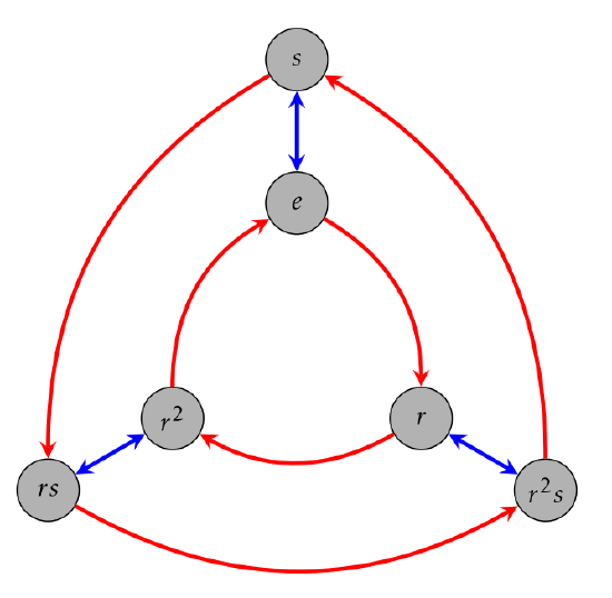
Definition 5.22: Cayley Diagram
Definition
We define the Cayley diagram\(C(G, S)\) of group \((G, \,\square\, )\) with generating set \(S\) as a directed graph where:
The vertices of \(C(G, S)\) are labelled by the elements of \((G, \,\square\, )\), i.e. \(V_{C(G,S)}:=G\)
Each edge of \(C(G, S)\) corresponds to a member \(s\) of the generating set \(S\); this edge is assigned the color \(c_s\) (multiple edges may correspond to the same \(s\in S\)). So our chromatic function satisfies \(f : E_{C(G,S)} \to S\)
An edge from \(g_1\) to \(g_2\) (\(\in G\)) exists if an only if \(g_2=g_1 \,\square\, s\), i.e. when \(g_2\) can be derived from \(g_1\) by operating on it and \(s\).
Chapter 5B - The Dihedral Groups
The dihedral group\(D_n\) is the group of symmetries of the regular \(n\)-gon.
Particularly, a regular \(n\)-gon in \(\mathbb{R}^2\) centered at \((0, 0)\) with vertices located at \(\displaystyle\left(\cos\left(\frac{2\pi k}{n}\right), \sin\left(\frac{2\pi k}{n}\right)\right)\) for \(k\in\set{0, 1, \dots, n-1}\)
The symmetries of the triangle and square are \(D_3\) and \(D_4\) respectively
\(D_n\) has order\(2n\), i.e. a regular \(n\)-gon has \(2n\) symmetries. We find \(n\) symmetries in the (convention: counter-clockwise) rotations\(r_k\) by \(\theta=k\dfrac{2\pi}{n}\) for \(k\in \set{0, 1, \dots, n-1}\) and \(n\) symmetries given by reflections: \(J_k\) for odd \(n\) and \(\tilde{J_k}\) for even \(n\).
If \(n\) is odd, each reflection passes through exactly one vertex and bisects the opposite edge of the \(n\)-gon. If \(n\) is even, a reflection passes through each vertex and bisects each edge. However, these lines of reflection "line up" such that they are double counted, so we have \(n\) of them.
Aside: I've come to learn that the notation \(D_n\) to mean the dihedral group of order \(n\) is non-standard; I won't change it, but be warned.
Subgroups of the Dihedral Groups
The dihedral groups have some basic subgroups:
The rotation \(r_1\) generates a cyclic subgroup\(R_n := \set{(r_1)^{k} \mid k\in\set{0, 1, \dots, n-1}}\) that consists of all the rotations in \(D_n\), so \(|R_n|=\dfrac{n}{2}\)
In general, the rotation \(r_a\) generates a cyclic subgroup of \(R_{n}\) (and thus of \(D_n\)) with order \(\dfrac{n}{\text{GCD}(a, n)}\).
So, \(R_n\) acts like \(\mathbb{Z}_n\)
For any reflection \(J_k\), \(\set{J_k, e}\) is a subgroup of order \(2\) because by the definition of a reflection, \(J_k ^2=e\).
Useful Identities for Computation
We can relate rotations and reflections with the identity \(\boxed{J_{k+1} = r^{k}J_1 r^{-k}}\) for odd \(n\) and \(\boxed{\tilde{J}_{k+1} = r^{k}\tilde{J}_1 r^{-k}}\) for even \(n\).
In terms of angles: \(\boxed{r_\theta J_0 r^{-1}_\theta=J_\theta}\).
Justification: this composition rotates \(\mathbb{R}^2\) counter-clockwise by \(k\) vertices, performs the "base" reflection about the \(0\)th vertex, then rotates back (clockwise) by \(k\) vertices again.
We also find that rotations followed by reflections are also reflections: \(\boxed{r^{k}J_1 = J_{\frac{\pi k}{n}}}\) for odd \(n\) and \(\boxed{r^{k}\tilde{J}_1 = \tilde{J}_{\frac{\pi k}{n}}}\) for even \(n\), \(\boxed{r_\theta J_0 = J_{\theta/2}}\).
\(J_\theta\) is the reflection about the line that forms angle \(\theta\) with the horizontal axis; we index \(J\) with its angle \(\theta\) instead of its corresponding integer for ease of notation.
Justification: \(r^{k}J_1\) cannot be a rotation (or \(J_1\) would be a rotation too), so it must be a reflection, and thus fix some line through \((0, 0)\). The other point fixed by \(r^{k}J_1\) is the point \(r^k\) sends \((1, 0)\), namely \(\displaystyle\left(\cos\left(\frac{\pi k}{n}\right), \sin\left(\frac{\pi k}{n}\right)\right)\), which trivially must be \(J_{\frac{\pi k}{n}}\).
We can also prove this by directly expanding out the definitions of the symmetries involved and evaluating the trigonometry.
Finally, from the general definition of the inverse of a composition, we find \(\boxed{J_{\theta_1}r_{\theta_2}=r^{-1}_{\theta_2} J_{\theta_1}}\). In the case \(\theta_1 = 0\), we find the useful identity \(\boxed{J_{0}r_{\theta_2}=r^{-1}_{\theta_2} J_{0}}\).
Chapter 5C - Homomorphisms and Isomorphisms
Definition 5.23: Group Homomorphism
Definition
A group homomorphism between groups \((G, \,\square\, )\) and \((H, \, \triangle )\) is a function\(\varphi : G \to H\) such that for \(g_1, g_2\in G\), \(\varphi(g_1 \,\square\, g_2)=\varphi(g_1)\, \triangle \, \varphi(g_2)\).
E.g. vector spaces are abelian groups under vector addition, so any linear transformation \(T: V_1 \to V_2\) is a group homomorphism since we know \(T(\vec{v}_1 + \vec{v}_2)=T(\vec{v}_1)+T(\vec{v}_2)\) holds for vector spaces (the inner \(\vec{v}_1 + \vec{v}_2\) happens in the vector space \(V_1\), whereas the righthand sum is in \(V_2\) because the vectors have already been transformed)
E.g. the determinant \(\det\) is a group homomorphism \(\det : \text{GL}_n(\mathbb{R}) \to (\mathbb{R}^\times, \cdot)\) because \(\det(AB)=\det(A)\det(B)\) for all \(A,B\in \text{GL}_n(\mathbb{R})\). Notably, \(\det\) only maps to the invertible elements of \(\mathbb{R}\), namely \(\mathbb{R}\setminus\set{0} =: \mathbb{R}^\times\).
E.g. the function \(\varphi : (\mathbb{Z}, +) \to (\mathbb{Z}_n, \, \boxplus \,)\) that maps \(\varphi(k) = [k]\) is a group homomorphism; this indicates that addition is well-defined between both groups. Note that its inverse is not a group homomorphism.
E.g. if \(G\) abelian, then \(\varphi : G \to G\) given by \(\varphi(a)=a^n\) for fixed \(n\in \mathbb{N}\) is a homomorphism (actually, an isomorphism, more later)
Generally, we just write \(\varphi(g_1 g_2)= \varphi(g_1)\varphi(g_2)\) to characterize a homomorphism; using the different symbols for binary operations illustrates that the implied operations act on different groups.
Thinking in terms of homomorphisms is useful everywhere in math because it lets you use what you know about one structure to learn about another structure.
Lemma 5.24: Homomorphism Identities
Lemma
If \(\varphi : G \to H\) is a homomorphism, then we have
\(\varphi(e_G)=e_H\), i.e. neutral elements are preserved under homomorphism
For all \(g\in G\), \((\varphi(g))^{-1}=\varphi(g^{-1})\), i.e. inverses are preserved under homomorphism.
If \(\psi : H \to K\) is also a group homomorphism, then \(\psi \circ \varphi\) is a group homomorphism
A monomorphism is an injective homomorphism.
If group \(G\) has subgroup \(H\), we have \(H \subseteq G\). The inclusion map\(\varphi : G \to H\) defined by \(\varphi(g)=g\) is a monomorphism.
Every monomorphism encodes an "inclusion" (more later)
A epimorphism is a surjective homomorphism.
E.g. \(\det : \text{GL}_n(\mathbb{R}) \to \mathbb{R}^\times\) is surjective, but not injective (e.g. there are multiple matrices with the same determinant).
E.g. \(\varphi : \mathbb{Z} \to \mathbb{Z}_n\) given by \(\varphi(a)=[a]\) is an epimorphism
Canonical example: the quotient group homomorphism
Definition 5.25: Group Isomoprhism
Definition
An isomorphism\(\varphi : G\to H\) is a group homomorphism between \(G\) and \(H\) that is both injective and surjective. Groups \(G\) and \(H\) are isomorphic iff there exists a group isomorphism between them.
An automorphism is an isomorphism from a group to itself, i.e. an isomorphism \(\varphi : G\to G\).
E.g. \(\varphi : D_3 \to S_3\) that maps a symmetry of an equilateral triangle to the corresponding permutation described by where it sends each of its corners, i.e. \(\varphi(S)=\begin{bmatrix}1 & 2 & 3 \\ S(1) & S(2) & S(3) \end{bmatrix}\) where \(S(i)\) is where vertex \(i\) is sent.
Isomorphic groups have the same shape, i.e. they are differently-named expressions of the same underlying structure. Any property a group can have (e.g. its order, whether it is abelian or cyclic, etc.) is invariant under isomorphism; thus, if two groups do not share a property, they cannot be isomorphic.
We can prove isomorphism by first providing (proving) a group homomorphism \(\varphi\), then
Directly proving that \(\varphi\) is both injective and surjective
Showing that \(\varphi\) has an inverse \(\varphi^{-1}\) that is a total function; this is effectively done by defining \(\varphi^{-1}\) explicitly.
Definition 5.26A: Kernel of a Homomorphism
Definition
The kernel\(\ker{\varphi}\) of group homomorphism \(\varphi : G\ \to H\) is the group of values that \(\varphi\) maps to the neutral element\(e_H\) of \(H\), i.e. \(\ker{\varphi} := \set{g \in G \mid \varphi(g)=e_H}\)
Definition 5.26B: Image of a Homomorphism
Definition
The image\(\text{Image}(\varphi)\) of group homomorphism \(\varphi: G \to H\) is the set of values in \(H\) that are mapped to from \(H\) by \(\varphi\), i.e. \(\text{Image}(\varphi) := \set{\varphi(g) \mid g\in G} = \set{h\in H \mid h = \varphi(g) \text{ for some } g\in G} \subseteq H\).
The (abuse of) notation \(\varphi(G)\) effectively suggests \(\text{Image}(G)\).
Lemma 5.27: Kernel and Images are Subgroups
Lemma
For homomorphism \(\varphi : G \to H\), \(\ker{\varphi}\) is a subgroup of \(G\) and \(\varphi(H) =: \text{Image}(H)\) is a subgroup of \(H\).
Lemma 5.28: Characterizing Homomorphism in terms of Kernel and Image
Lemma
Group homomorphism \(\varphi : G \to H\) is injective if and only if \(\ker{\varphi}=\set{e_G}\) and surjective if and only if \(\text{Image}(\varphi)=H\). \(\varphi\) is an isomorphism if and only if both of these conditions hold.
Proof (injectivity): \(\implies\): as a homomorphism, \(\varphi\) must map \(g\) to \(e_H\) if \(g\in \ker{\varphi}\); homomorphisms map neutral elements to neutral elements, so \(\varphi(g)= \varphi(e_G)\). We assumed injectivity, so this implies \(g=e_G\), implying \(\ker{\varphi}=\set{e_G}\). \(\impliedby\): if \(\varphi(g_1)=\varphi(g_2)\), then \(\varphi(g_1)\varphi(g_2)^{-1}=e_H\), so \(\varphi(g_1)\varphi(g_2^{-1})=\varphi(g_1 g_2^{-1})=e_H\) since \(\varphi\) is a group homomorphism. Thus, \(g_1 g_2^{-1}\in \ker{\varphi}\), and thus is equal to \(e_G\) by assumption. Thus, \(g_1=g_2\).
Proof (surjectivity): we are just restating the definition of subjectivity here.
Lemma 5.29
Lemma
For group \(G\) with element \(g\in G\), if \(g^k=e_G\), then \(o(g) \mid k\), i.e. \(k\) is a multiple of \(o(g)\), the order of \(g\) in \(G\).
E.g. for abelian group \(G\), \(\varphi: G \to G\) given by \(\varphi(g)=g^k\) is a group homomorphism with kernel \(\set{g\in G \mid g^k=e}\). We can use a number-theoretic argument to derive \(o(g) \mid k\); this is good example to generalize the previous lemma from
E.g. for homomorphism \(\varphi: \mathbb{Z}_n \to \mathbb{Z}_n\) given by \(\varphi([a])=k[a]\) for some \(k\), then \(\ker{\varphi}=\set{[a]\in \mathbb{Z}_n \mid k[a]=[0]}\), which implies that \(o(a)\mid k\), implying \(|\langle [a] \rangle| \mid k\). We know \(\langle [a] \rangle = \langle [ \text{GCD}(a, n) ] \rangle\), which has order \(\frac{n}{\text{GCD}(a, n)}\), so \(\frac{n}{\text{GCD}(a, n)}\mid k\). So, \(\ker{\varphi} = \set{[a] \in \mathbb{Z}_n \mid \frac{n}{\text{GCD}(a, n)} \text{ divides } k}\).
Also, \(\varphi(a)=k[a]=[ka]=a[k]\), so \(\text{Image}(\varphi)=\set{[a] \mid a \in \mathbb{Z}} := \langle [k] \rangle\). This is useful even when we don't know the value of \(k\); all group homomorphisms \(\varphi: \mathbb{Z}_n \to \mathbb{Z}_n\) can be expressed as \(\varphi([a])=k[a]\) (earlier result).
Lemma 5.30: Inverse of Isomorphism is an Isomorphism
Lemma
If \(\varphi :G \to H\) is an isomorphism, then it is invertible and its inverse \(\varphi^{-1} : H \to G\) is also an isomorphism.
Moreover, we can show that a homomorphism \(\varphi\) is an isomorphism by showing that \(\varphi^{-1}\) is a homomorphism as well.
Proposition 5.31: Classification of Cyclic Groups
Proposition
For cyclic group \(G\) generated by element \(a\), i.e. \(\langle a \rangle\):
If \(a\) has finite order, then \(G\) is isomorphic to \(\mathbb{Z}_{o(a)}\)
If \(a\) has infinite order, then \(G\) is isomorphic to \(\mathbb{Z}\) (\(=: \mathbb{Z}_\infty\) by abuse of notation)
We propose the isomorphism \(\varphi : (\mathbb{Z}_n, +) \to G\) defined by \(\varphi([k])=a^k\) to prove both facts. In each case, we must prove that \(\ker{\varphi}=[0]\) and \(\text{Image}(\varphi)=G\).
So, cyclic groups "look like" the integers mod \(n\) for \(n\in \mathbb{N}\cup \set{\infty}\)
A useful way to show non-isomorphism is to consider the order of all the element in one group and show that no element of that order exists in another. E.g. \(\mathbb{Z}_4\) has elements of order \(4\), but \(\mathbb{Z}_2 \times \mathbb{Z}_2\) doesn't.
Chapter 5D - Cosets and Lagrange's Theorem
Definition 5.32: Left and Right Cosets
Definition
Let \(G\) be a group with element \(a\) and subgroup \(H\). The left coset\(aH\) of \(a\) in \(H\) is defined as \(aH := \set{ah \mid h\in H}\subseteq G\). The right coset\(Ha\) of \(a\) in \(H\) is \(Ha := \set{ha \mid h\in H}\subseteq G\).
E.g. \(eH = He = H\) in general
E.g. for \(G=(\mathbb{Z}, +)\) and \(H=4\mathbb{Z}\), the cosets are \(n + 4\mathbb{Z}\) for \(n\in \set{1, 2, 3, 4}\)
E.g. for \(G=S_3, H=\set{\text{id}, (1, 2)}\), we have \((2, 3)H = \set{(2, 3), (2, 3) \circ (1, 2)}=\set{(2, 3), (1, 3, 2)}\), which also happens to be equal to \((1, 2, 3)H\). Funny…
We usually consider left cosets
Proposition 5.33: A group is the union of its cosets under any subgroup
Proposition
Let \(G\) be a group with subgroup \(H\).
For all \(a, b\in G\), either \(aH = bH\) or \(aH \cap bH=\emptyset\); the same fact is true of right cosets
\(G\) is equal to the (disjoint) union of all its left (or right) cosets of \(H\) in \(G\), i.e. \(\displaystyle G = \bigcup_{g\in G} gH = \bigcup_{g\in G} Hg\).
Proof (first): Assume \(aH \cap bH\ne \emptyset\), so pick \(c \in aH \cap bH\). So, \(c=ah_a=bh_b\). From this we get \(ah_a=bh_b\implies b=ah_a h_b^{-1}\). So, if \(bh\in bH\), then \(bh=ah_a h_b^{-1}\in aH\), so \(bH \subseteq aH\). We can make exactly the same argument switching \(aH\) for \(bH\). So, \(bH=aH\).
Proof (second): \(a\in G\implies a\in aH\implies a \in \bigcup\limits_{g\in G} gH\), so this is a superset of or equal to \(G\). Clearly each element in the union is in \(G\), so this union is equal to \(G\).
Theorem 5.34: Lagrange's Theorem (Coset version)
Theorem
Let \(G\) be a finite group with subgroup \(H\). Then the order \(|H|\) of \(H\) divides the order of \(|G|\) (as we know). Also, the number of left cosets of \(H\) in \(G\) is equal to \(\dfrac{|H|}{|G|}\).
Proof: by proposition 5.33, we know that there exist disjoint cosets \(a_1H, \dots, a_n H\) whose union forms \(G\). So, \(|G| = |a_1 H| + \dots + |a_n H|\). We also know from our theory of cosets that \(H \mapsto a_i H\) is a bijection for all \(i\), so \(|a_i H|=|H|\) for each \(0 \leq i \leq n\). Thus, \(|G| = |H| + \dots + |H|\) (\(n\) times) \(=n|H|\). Thus, we know that \(|H|\) divides \(|G|\). We implicitly defined \(n\) as the number of left cosets, so \(n=\dfrac{|G|}{|H|}\), as desired.
We define the index\([G : H]\) of subgroup \(H\) of group \(G\) as the number of left cosets of \(H\) in \(G\). Thus, by Lagrange's Theorem, \([G : H] = \dfrac{|G|}{|H|}\).
Corollary 5.36: Order of an Element divides the Order of a Group
Corollary
For finite group \(G\) with element \(a\in G\), the order of \(a\) in \(G\) divides the order of \(G\) (i.e. \(o(a) \mid |G|\)) and \(\boxed{a^{|G|}=e}\).
Proof: we know that \(\langle a \rangle\) must be a subgroup of \(G\) (namely, a cyclic subgroup). So, by Lagrange's theorem, \(| \langle a \rangle | =: o(a)\) divides \(|G|\). Thus, \(|G|=k \cdot o(a)\) for integer \(m\); we have \(A^{|G|}=a^{o(a) \cdot m}=(a^{o(a)})^m=e^{m}=e\), i.e. since \(o(a)\) divides \(|G|\), \(|G|\) is a multiple of \(o(a)\) and thus is like "returning back to \(e\) through \(\langle a \rangle\)" multiple times.
Corollary (#1) 5.37: Subgroups of Group of prime order
Corollary
Let \(G\) be a group of prime order, i.e. \(|G| = p\) for prime some \(p\)
The only subgroups of \(G\) are \(G\) itself and the trivial subgroup\(\set{e}\)
All non-identity elements of \(G\) generate \(G\), i.e. for \(a\in G\), \(a \ne e\implies G = \langle a \rangle\)
\(G\) is isomorphic to \(\mathbb{Z}_p\)
Proof: The order of any subgroup must divide the order of the group; since this is prime, subgroups could only be of size \(1\) or \(p\). We have described both; these must be the only subgroups (1). So, if \(a\ne e\), then \(\langle a \rangle\) doesn't generate a subgroup \(\implies\) it must generate \(G\) (2). (3) follows from theorem 5.16.
Aside: where does the definition of "prime" come from? Ring theory, or can it be defined entirely within group theory?
Aside: this seems connected to the "All fields of prime order are the same" Galois field thing from MATH 422
Left and right cosets of a group are different in general, but might be the same for certain subgroups. A normal subgroup is a subgroup \(H\) of group \(G\) such that the right cosets of \(H\) in \(G\) are equal to the left cosets of \(H\) in \(G\).
Definition 5.38: Normal Subgroup
Definition
A normal subgroup\(N\) of \(G\) (denoted \(N \unlhd G\)) is some subgroup \(N\) such that, for all \(g\in G\), we have \(gNg^{-1} := \set{gng^{-1} \mid n\in N} \subseteq N\). This implies that for all \(n\in N\) and \(g\in G\), we have \(gng^{-1}\in N\) as well.
E.g. the subgroup of \(\text{GL}_n(\mathbb{F})\) consisting of all matrices with determinant \(1\) (called the special linear group\(\text{SL}_n(\mathbb{F})\)) is normal. This inherits from the fact that the determinant is a group homomorphism, and thus that the product of determinants of inverse matrices is \(1\).
Generally, a special group of matrices has determinant \(1\) (more examples following this naming convention exist)
Any "rotation subgroup" \(R_n \cong \mathbb{Z}_n\) of dihedral group \(D_n\) is normal (informally) because the composition of rotations is a rotation and two flips cancel out to being a rotation again.
We could also say "subgroup \(N\) is closed under conjugation by \(G\)"
When the set of right cosets and left cosets equal, we use the notation \(G/N\) to denote the set of cosets that normal subgroup \(N\) of \(G\) induces on \(G\).
This is a quotient, which denotes set of cosets of a group. We will learn that this is also a group that "sands away / congeals" the structure of the normal subgroup within the parent group.
If \(G\) is Abelian, then all of its subgroups are trivially normal. This might provide some insight into what "flavour" normal groups have.
Corollary (#2) 5.39
Corollary
If \(G\) is an abelian group generated by \(2\) elements \(a, b\) with orders \(p,q\) where \(p\) and \(q\) are distinct primes, then the order of \(G\) is \(p\times q\).
Proof: every element in \(G\) can be written as \(a^{i}b^{j}\) for \(i \in \set{0, \dots, p-1}\) and \(j\in \set{0, \dots, q-1}\). So, \(G\) can have at most \(p\times q\) elements (it could be smaller if there is "overlap" of the terms). By the first corollary of Lagrange's theorem, \(p\) and \(q\) must both divide \(|G|\); since \(p, q\) are distinct primes, \(\text{GCD}(p, q=1)\) so \(p\times q\) must divide \(G\), i.e. \(|G|\) must be at least \(p\times q\). Thus, \(|G|=p\times q\).
This trivially extends to a group generated by any number of distinct primes
Proposition 5.40: Kernels of Homomorphisms are Normal Subgroups
Proposition
If \(G\) is a group with subgroup \(H\) and \(\varphi : G\to H\) is a homomorphism from \(G\) to \(H\), then \(\ker{\varphi}\) is a normal subgroup of \(G\).
Proof: for \(a\in \ker{\varphi}\) and \(g\in G\), \(\varphi(gag^{-1})=\varphi(g)\varphi(a)\varphi(g^{-1})=\varphi(g)e_H \varphi(g)^{-1}=e_H\). Thug, \(gag^{-1}\in \ker{\varphi}\). So, it follows from the fact that homomorphisms preserve inverses, which cancel out
The kernels of group homomorphisms provide good examples of normal subgroups
E.g. we define the sign homomorphism\(\varepsilon : S_n \to (\set{\pm 1}, \times)\) that checks the parity of how many transpositions define a permutation, i.e. \(\varepsilon : (\tau_k \dots \tau_2 \tau_1) \mapsto (-1)^k\).
We define \(\ker{\varepsilon}\) as the alternating group\(A_n\); it is subgroup of permutations that can be constructed as the product of an even number of transpositions. By proposition 5.40, it is a normal subgroup.
Thus, \({S_n}/({\set{\pm 1}, \times})\cong A_n\); this is suggestive of what we will see in the next chapter
Chapter 5E - The Quotient Construction and Noether's Isomorphism Theorems
For group \(G\) with normal subgroup \(N\), we have seen the set \(G/N\) of cosets induced by \(N\) in \(G\). It turns out that the set \(G/N\) is amenable to being a group; we just have to determine the right operation to define over it. This is known as the quotient construction; \(G/N\) is a quotient group under this operation.
We also adopt the notation \(\overline{a} := aN\) to denote the coset of \(N\) associated with \(a\) where \(N\) is clear based on context.
Theorem 5.41: Quotient Construction
Theorem
For group \(G\) with normal subgroup \(N\), we can define a unique product over the set \(G/N\) of cosets of \(N\) in \(G\) that makes it a group. Further, the function \(\gamma : G\to G/N\) that maps an element of \(G\) to its coset induced by \(N\) (i.e. defined by \(\gamma(a):=aN\)) is a group homomorphism.
Proof that \(\gamma\) is well-defined: let \(a, a_1, b, b_1 \in G\) by arbitrary such that \(\overline{a}=\overline{a_1}\) and \(\overline{b}=\overline{b_1}\). So, \(a_1 =an_1\) for some \(n_1\in N\), and thus \(a_1 b = an_1 b= a (bb^{-1})n_1 b\) (insertion) \(=ab(b^{-1}n_1b)\). \(N\) is a normal subgroup, so \(n_2 := b^{-1}n_1b \in N\), and thus \(ab(b^{-1}n_1 b)=abn_2 \in abN\) by definition (i.e. \(\in \overline{ab}\)). Thus, \(\overline{a_1 b}=\overline{an_1 b}=\overline{ab}\), proving well-definedness for \(a\). For \(b\), if \(\overline{b}=\overline{b_1}\), then \(bN=b_1 N \implies abN=ab_1 N\)\(\implies \overline{ab}=\overline{ab_1}\). Thus, \(\gamma\) is well-defined.
It is routine to show that \(G/N\) is a group under the binary operation \(\square\, : (\overline{a}, \overline{b}) \mapsto\overline{ab}\), and that \(\gamma\) is a group homomorphism
Informally, we can give the cosets of \(G\) by implied by \(N\) a group structure by defining a homomorphism \(\gamma\) from \(G\) that "adapts" \(G\)'s operation to \(G/N\). Specifically, to operate on two elements of \(G/N\), we pick arbitrary members from the corresponding cosets and use \(G\)'s operation on those, then take that element's coset.
We say an operation is well-defined if it is a group epimorphism (surjective homomorphism), since this suggests some sort of "many-to-one" mapping like a coset or equivalence class. Importantly, if an operation is well-defined, we can chose any representatives from the classes over which it is defined and get the same result.
E.g. \(\mathbb{Z}/{2\mathbb{Z}}\) is a quotient group since \(\mathbb{Z}\) is abelian → all subgroups are normal. \([\mathbb{Z} : 2 \mathbb{Z}]=2\), so \(\mathbb{Z}/2\mathbb{Z}\) has \(2\) elements (aside: why is the index equal to the order of the quotient group? we'll see…). In particular, \(\mathbb{Z}/2\mathbb{Z}\) is isomorphic to \(\mathbb{Z}_2\); we can see this with the mapping \(\overline{0}\mapsto [0], \overline{1}\mapsto [1]\).
In general, \(\mathbb{Z}/n\mathbb{Z}\) is isomorphic to \(\mathbb{Z}_n\), with isomorphism \(\varphi : \overline{a}\mapsto [a]\). The proof is straightforward.
Theorem 5.42: Factorization Theorem
Theorem
Let \(\varphi :G \to H\) be a group homomorphism between groups \(G\) and \(H\). Let \(N\) be a subgroup of \(\ker{\varphi}\) that is normal in \(G\), i.e. \(N \unlhd G\). Let \(\gamma : G \to G/N\).
Then there exists a homomorphism \(\overline{\varphi}: G/N \to H\) such that \(\varphi := \overline{\varphi}\circ \gamma\).
Informally, the factorization theorem suggests that if we have a homomorphism \(\varphi : G \to H\), the structure of the homomorphism is preserved if we take the quotient with respect to some normal subgroup \(N\) of \(\ker{\varphi}\) "first". Specifically, it states we can find another homomorphism from \(G/N\) to the subgroup \(H\).
Since \(N\) also "depends" on the definition of \(\varphi\), the structures "line up" so that nothing about the relationships between the cosets are changed.
We can illustrate the factorization theorem with the following commutative diagram
\usepackage{tikz-cd}\begin{document}\begin{tikzcd}[scale=5] G \arrow[r, "\varphi"] \arrow[d, "\gamma"'] & H \\ G/N \arrow[ru, "\overline{\varphi}"']\end{tikzcd}\end{document}
Theorem 5.43: First Isomorphism Theorem
Theorem
Let \(\varphi :G \to H\) be a group homomorphism between groups \(G\) and \(H\). Let \(N\) be a subgroup of \(\ker{\varphi}\) that is normal in \(G\), i.e. \(N \unlhd G\). Let \(\gamma : G \to G/N\). (same as factorization thm assumptions).
If \(N=\ker{\varphi}\), then \(\tilde{\varphi}\) is an isomorphism between \(G/\ker{\varphi} \to H\).
Note: if \(\varphi\) is surjective, then \(\text{Image}(\varphi)=H\) and \(\tilde{\varphi} : G/\ker{\varphi}\to H\) is an isomorphism.
More succinctly, the First Isomorphism Theorem states that \(G/\ker{\varphi} \cong H\) for any \(\varphi : G \to H\). It is a special case of the Factorization Theorem, i.e. when \(H = \ker{\varphi}\) (which is know is normal). Intuitively, the structure of \(\ker{\varphi}\) is the same as the internal structure of the cosets of \(H\). So, taking the quotient doesn't "remove any detail" about the structure of the cosets of \(H\), just the "detail" within the cosets.
E.g. Define the homomorphism \(\varphi : \mathbb{Z}\to \mathbb{Z}_n\) as \(\varphi(k)=[k]\). \(\varphi\) is surjective and \(\ker{\varphi}=n \mathbb{Z}\). By the first isomorphism theorem, \(\mathbb{Z}_n\) is isomorphic \(\mathbb{Z}/n \mathbb{Z}\). Moreover, by the factorization theorem, \(\overline{\varphi}: \mathbb{Z}/ n \mathbb{Z} \to \mathbb{Z}_n\) given by \(\overline{\varphi}(\overline{k})=[k]\) is an isomorphism since \(\overline{\varphi}(\overline{k})=\overline{\varphi}(\gamma(k))=\varphi(k)=[k]\).
E.g. if \(T\) is the group of affine transformations and \(B\) is the group of translations. We define the homomorphism \(\varphi : T \to \text{GL}_n(\mathbb{R})\) that simply considers the invertible matrix part of the affine transformation (and discards the translation). Clearly, \(\ker {\varphi}\cong B\), so by the First Isomorphism Theorem, \(G/T \cong \text{GL}_n(\mathbb{R})\).
Theorem 5.44: Correspondence Theorem
Theorem
Let \(G\) be a group with normal subgroup\(N\)
If \(N \unlhd H \leq G\) (i.e. \(H\) is a subgroup of \(G\) that contains \(N\)), then \(\gamma\) maps \(H\) to \(H/N\) and \(H/N\) is a subgroup of \(G/N\). Furthermore, if \(H\) is normal in \(G\), then \(H/N\) is normal in \(G/N\).
I.e. \(\gamma(H)=H/N\) is normal in \(G/N\).
If \(K\leq G/N\) (i.e. \(K\) is a subgroup of \(G/N\)), then \(\gamma^{-1}(K)\) is a subgroup of \(G\) that contains \(N\), i.e. \(N \unlhd \gamma^{-1}(K)\leq G\). Furthermore, if \(K\) is normal in \(G/N\), then \(\gamma^{-1}(K)\) is normal in \(G\). Here, \(\gamma^{-1}(K) = \set{a \in G \mid \gamma(a)\in K}\).
Proof (1): \(\gamma(H)\) must be a subgroup of \(G/N\). \(H\) is normal in \(G\), so for \(g\in G\) and \(h\in H\), we have \(\overline{g}\overline{h}\overline{g}^{-1}=\overline{g}\overline{h}\overline{g^{-1}}=\overline{ghg^{-1}}\). We know \(ghg^{-1}\in H\), so \(\overline{ghg^{-1}} \in H/N=\gamma(H)\). So \(H/N\) is normal in \(G/N\); the proof more or less inherits from well-definedness.
Proof (2): Again, \(\gamma^{-1}(K)\) must be a subgroup of \(G\) because \(\gamma\) is a homomorphism. For \(g\in G\) and \(a\in \gamma^{-1}(K)\), we have \(gag^{-1}\in \gamma^{-1}(K)\iff \gamma(gag^{-1})\in K\iff \gamma(g)\gamma(a)\gamma(g^{-1})\in K\iff \overline{g}\overline{a}\overline{g^{-1}}\in K\). \(K\) is normal by assumption, so the first assumption must hold; \(\gamma^{-1}(K)\) is normal.
Intuition: through the factorization and first isomorphism theorems, we learned how \(\gamma\) and \(\varphi\) interact together on elements of \(G\). The correspondence theorem examines what happens to the structure of entire subgroups of \(G\).
When \(\varphi : G \to G/N\) is a homomorphism for subgroup normal \(N\) of \(G\) and we have \(H\) such that \(N \unlhd H \leq G\), it turns out \(\gamma(H)=H/N\), i.e. the quotient gets applied to subgroup \(H\) just like it does to subgroup \(G\). So, a given subgroup \(H\) of \(G\)corresponds to a subgroup \(H/N\) of \(G/N\).
The second part suggests that this happens in reverse: if \(K\) is some subgroup of \(H/N\), then \(\gamma^{-1}(K)\) will be a subgroup of \(G\) that contains \(N\) as a normal subgroup. In this sense, \(\gamma^{-1}\) "gives back" the structure of the full group from the quotient; \(N\) gets "expanded" out from "nothing".
We also see that "normality" is preserved by \(\gamma\).
Theorem 5.45: Second Isomorphism Theorem
Theorem
Let \(N \unlhd G\) and \(H \leq G\). Then,
\(\gamma(H)=\gamma(HN)=HN/N\).
\(\gamma(H)\cong H/(H\cap N)\)
So, the second isomorphism theorem tells us what the structure a subgroup \(H\) will have when mapped from \(G\) to quotient \(G/N\) by \(\gamma\).
Intuition: We know from the correspondence theorem that \(\gamma(H)\) is a subgroup of \(G/N\); the second isomorphism theorem gives us more information about its structure, namely that it is isomorphic to \(H/(H\cap N)\).
It also states that \(\gamma(H)=\gamma(HN)\); intuitively, since \(\gamma\) performs a quotient by \(N\), "multiplying" by \(N\) here won't make a difference.
Theorem 5.46: Third Isomorphism Theorem
Theorem
Let \(N \unlhd H \unlhd G\) (where we also have \(N \unlhd G\)). Then \((G/N)/(H/N)\cong G/H\).
The Third Isomorphism Theorem tells us that quotients of groups act in the same way as division: taking the quotient by \(N\) of both terms of a different quotient (\(G/H\)) will yield an isomorphism.
Intuitively, if \(N\) is normal subgroup of both \(G\) and \(H\), then the structure "wiped away" by \(N\) is shared by both \(G\) and \(H\), so it would also by "wiped away" by the quotient \(G/H\) as well.
Chapter 6 - Finite Abelian Groups and Semi-direct Products
We define the direct product\(G\times H\) of groups \(G\) and \(H\) as \(\set{(g, h) \mid g\in G, h\in H}\).
Specifically, for \((G, \cdot)\) and \((H, \star)\), we have \((g_1, h_1) * (g_2, h_2) := (g_1\cdot g_2, h_1 \star h_2)\)
Identity: \((e_G, e_H)\)
Inverse: \((g^{-1}, h^{-1})\)
E.g. the vector space \(\mathbb{R}^2\) is the direct product \(\mathbb{R} \times \mathbb{R}\)
E.g. If we define \(S^1\) as the group of rotations of the plane (under composition), then \(S^1\times S^1\) is a group isomorphic to a 2D torus.
Expressing a group as the direct product of other groups gives insights into its structure.
Theorem 6.2
Theorem
If \(n\in \mathbb{N}\) decomposes into prime factors \(n=p_1^{e_1} p_2^{e_2}\dots p_r ^{e_r}\) where any two \(p\) terms are distinct, then \(\mathbb{Z}_n \cong \mathbb{Z}_{p_1^{e_1}} \times \mathbb{Z}_{p_2^{e_2}} \times \dots \times \mathbb{Z}_ {p_r^{e_r}}\).
Note: we may have \(\mathbb{Z}_{p^{e_1}}\times \mathbb{Z}_{p^{e_2}} \not\cong \mathbb{Z}_{p^{e_1 + e_2}}\). E.g. \(\mathbb{Z}_4 \not\cong \mathbb{Z}_2 \times \mathbb{Z}_2\). This is clear from the orders of the subgroups in each group
Proof relies on applying first isomorphism theorem to the homomorphism \(\varphi : \mathbb{Z} \to \mathbb{Z}_{p_1^{e_1}} \times \mathbb{Z}+{p_2^{e_2}} \times \dots \times \mathbb{Z}_ {p_r e^r}\) given by \(\varphi(k)=([k]_{p_1 ^{e_1}}, [k]_{p_2 ^{e_2}}, \dots, [k]_{p_k ^{e_k}})\)
Chinese remainder theorem: For distinct primes \(p_1, p_2\) and \(a, b \in \mathbb{Z}\), there exists \(x\in \mathbb{Z}\) such that \(x \equiv a \mod p_1^{e_1}\) and \(x \equiv b (\mod p_2^{e_2})\)
Theorem 6.4: Classification Theorem for Finite Abelian Groups
Theorem
Every finite abelian group is isomorphic to a direct product of cyclic groups whose orders are prime powers. I.e. any finite abelian \(G\) is isomorphic to \(\mathbb{Z}_{p_1 ^{e_1}} \times \mathbb{Z}_{p_2 ^{e_2}} \times \dots \times \mathbb{Z}_{p_r ^{e_r}}\). For not necessarily distinct primes \(p_1, p_2, \dots p_r\).
The order of this group is clearly \(p_1^{e_1} \times p_2^{e_2} \times \dots \times p_r^{e_r}\). So, the property of \(|G|\in \mathbb{N}\) needing to be decomposable into prime factors also applies to \(G\) as well (so \(G\mapsto |G|\) is some kind of homomorphism).
To find all the possible finite abelian groups of a given order (e.g. \(360\) for this example), we:
Find the prime factors of the order: \(360 = 2^{3}\times 3^{2} \times 5\).
Find every way to write the factored expression as a product of prime powers (with at least one different term): \(8 \times 9 \times 5\), \(4\times 2\times 9\times 5\), \(2\times 2\times 2\times 9\times 5\), \(8 \times 3\times 3 \times 5\), \(4\times 2\times 3\times 3\times 5\), \(2\times 2\times 2\times 3\times 3\times 5\).
These correspond to the possible decompositions into cyclic groups
Corollary 6.5: Cauchy's Theorem for Finite Abelian Groups
Corollary
if \(G\) is a finite abelian group and prime \(p\) divides \(|G|\), then \(G\) has a subgroup of order \(p\).
Proof sketch: the structure of \(G\) must be isomorphic to some \(\mathbb{Z}_{p_1 ^{e_1}} \times \mathbb{Z}_{p_2 ^{e_2}} \times \dots \times \mathbb{Z}_{p_r ^{e_r}}\) by THM 6.4, so for any prime \(p\) that divides \(|G|\) must be equal to some \(p_i\) in the decomposition. A subgroup of \(\mathbb{Z}/{p_i^{e_i}} \mathbb{Z}\) of order \(p\) is generated by \(\overline{p_i ^{e_i -1}}\), since the order of this subgroup must divide \(p\) → is \(p\). So, the subgroup \(\langle \overline{p_i ^{e_i -1}} \rangle \times \set{\overline{0}} \times \dots \times \set{\overline{0}}\) of \(G\) is over order \(p\).
Theorem 6.6
Theorem
For prime \(p\), \(\Phi(p)\) (the group over invertible elements of \(\mathbb{Z}_p\) under multiplication) is cyclic and of order \(p-1\). Thus, it is isomorphic to \(\mathbb{Z}_{n-1}\).
Theorem 6.7: Structure Theorem of \(\Phi(n)\)
Theorem
For \(\mathbb{N}\ni n =p_1^{e_1} \times p_2^{e_2} \times \dots \times p_r^{e_r}\), we have \(\Phi(n)\cong \Phi(p_1^{e_1}) \times \Phi(p_2^{e_2}) \times \dots \times \Phi(p_r^{e_r})\).
For any \(p_i\ne 2\), then \(\Phi(p^e)\) under \(\times\) is isomorphic to \(\mathbb{Z}_{p^{e-1}\times (p-1)}\) under addition (and thus cyclic).
The idea of decomposing a group into a direct product of simpler groups is helpful, but the direct product is only defined for finite abelian groups. The semi-direct product generalizes this concept to non-abelian groups.
Definition 6.8: Semi-direct Product
Definition
Let \(G\) be a group with subgroups \(N, A\) where \(N \unlhd G\) and \(N \cap A=\set{e}\). Furthermore, assume \(G=NA\), i.e. any \(g\in G\) is equal to \(na\) for \(n\in N\), \(a\in A\). Then, \(G\) is the semi-direct product\(N\rtimes A\) of \(N\) and \(A\).
E.g. \(S_n = A_n \rtimes \set{\text{id}, (1,2)}\) where \(A_n\) is the alternating group.
Chapter 7 - Group Actions
A group action on a set takes one member of the set and maps it to another in a way that mirrors the structure of the group. So, a group action "applies" the structure of a group to the set. Actions are defined when the structure of the set is compatible with that of the group.
Recall that for a set \(X\), the set of bijections \(f : X \to X\) is a group under composition denoted \(\text{Sym}(X)\).
Definition 7.2: Group Action
Definition
An action of group \(G\) on a set \(X\) is a homomorphism \(\varphi: G \to \text{Sym}(X)\).
An action of \(S_n\) on \(\set{1, 2, \dots, n}\) permutes the numbers \(1, 2, \dots, n\).
An action of \(D_n\) on the set of vertices of a regular \(n\)-gon transforms the \(n\)-gon in a way that preserves its structure
An action of \(\text{GL}_n({\mathbb{R}})\) acts on the set of vectors \(\mathbb{R}^n\) by matrix-vector multiplication
A group may act on itself (i.e. when the set \(X\) being acted upon is \(G\) itself) or the set of its own subgroups. Common self-actions include
Left multiplication: for \(a \in G\), \(g\in G\) acts on \(a\) by multiplying it on the left: \(g(a) := ga\)
Conjugation: for \(a \in G\), \(g\in G\), \(g(a) := gag^{-1}\)
Subgroup conjugation: for subgroup \(H\) of \(G\), \(g\in G\) acts on \(H\) by \(g(H):=gHg^{-1}\).
Theorem 7.3: Cayley's Theorem
Theorem
Any finite group \(G\) is isomorphic to a subgroup of \(S_n\).
Proof: we know a homomorphism \(\varphi : G \to \text{Sym}(G)\) given by left multiplication exists. Trivially, we can show \(\ker{\varphi}=\set{e}\) → \(\varphi\) is an isomorphism → \(G\cong \text{Sym}(G)\) → \(G\cong S_{|G|}\).
Definition 7.4: Orbits
Definition
Let group \(G\) act on set \(X\) and fix \(x\in X\). The orbit\(\mathcal{O}(x)\) of \(x\) is the set of all the elements of \(X\) that can be reached from \(x\) by applying an action of \(G\), i.e. \(\mathcal{O}(x):=\set{g(x) \mid g\in G}\).
E.g. if \(G\) is the set of rotations in \(\mathbb{R}^2\) (i.e. \(\text{SO}_2{(\mathbb{R})}\)) and \(X\) is \(\mathbb{R}^2\), then the orbit of element \(\vec{x}\in X\) is set of points with distance \(\| \vec{x} \|\) from the origin, i.e. \(\mathcal{O}(\vec{x})\) is the circle of radius \(\| \vec{x}\|\).
E.g. if \(G\) is \(S_n\) and \(X\) is \(\set{1, 2, \dots, n}\), then the orbit of any element in \(X\) is trivially \(\text{Sym}(X)\).
E.g. if \(G\) acts on the set of its own subgroups by left-multiplication, the orbit of \(x\in G\) is the right coset \(Hx\)
The conjugacy class of \(h \in G\) set of \(\set{ghg^{-1}\mid g\in G}\). So, the conjugacy class of \(h\in G\) is its orbit under \(G\) acting on itself by conjugation.
Any two orbits are either equal or disjoint; so orbits partition the set \(X\) (and thus imply an equivalence relation over \(X\)). (Proposition 7.5).
An orbit is transitive if there is only one orbit (which contains every element of \(X\)). (Definition 7.6)
Let group \(G\) act on set \(X\). The stabilizer\(\text{Stab}(x)\) of \(x\in X\) is the set \(\set{g\in G \mid g(x)=x}\), i.e. the set of actions in \(G\) that send the element \(x\in X\) to itself. The stabilizer is a subgroup of \(G\).
If \(G\) acts on itself by conjugation, we call this set the centralizer of \(G\)
If \(G\) acts on the set of its own subgroups by conjugation, we call this set the normalizer of \(G\).
E.g. if \(G\) acts on itself by left-multiplication, then for any \(x\in G\), \(\text{Stab}(x)=\set{e}\).
E.g. if \(G\) is the set of symmetries of the cube and \(X\) is the set of vertices of the cube, the stabilizer of action of some vertex \(x\in X\) is the set of actions in \(G\) that don't move that vertex
E.g. if \(G\) is \(S_n\) acting on \(X=\set{1, 2, \dots n}\), then the stabilizer of some permutation number \(x\in X\) is the set of permutation in \(S_n\) that fix \(x\).
Theorem 7.8: Orbit-Stabilizer Theorem
Theorem
Let group \(G\) act on set \(X\) and fix \(x\in X\). Then, the function \(\psi : G/\text{Stab}(x)\to \mathcal{O}(x)\) given by \(\psi(\overline{g}(x)) \mapsto g(x)\) is a bijection.
\(\text{Stab}(x)\) is not necessarily normal, so \(G/\text{Stab}(x)\) might not be a group itself. However, if it is, then \(\psi\) is an isomorphism.
Proof: First we show that \(\psi\) is well-defined. Let \(\varphi : G \to \mathcal{O}(x)\), \(\varphi(g)=g(x)\) and \(g,\tilde{g}\) be in the same coset of \(G\) by \(\text{Stab}(x)\). We have \(\varphi(g)=g(x)\); \(g(x)=\tilde{g}(h(x))\) (for some \(h\in \text{Stab}(x)\)) \(= \tilde{g}(x)\) (by defn of \(\text{Stab}(x)\)) \(=\varphi(\tilde{g})\), so \(\psi\) is well-defined. Since \(g\) is arbitrary in the theorem, \(\psi\) is clearly surjective. By factorization theorem, \(\varphi = \psi \circ \gamma\) (where \(\gamma : G \to G/\text{Stab}(x)\)). So, \(\psi(\gamma(g))=\varphi(g)=g(x)\) and thus \(\psi(g)=g(x)\). Finally, \(\psi(\overline{g_1})=\psi(\overline{g_2})\implies g_1(x)=g_2(x)\implies g_2^{-1}g_1(x)=x \implies g_2^{-1}g_1\in \text{Stab}(x)\). So, \(g_1=g_2 h\) for some \(h\in \text{Stab}(x) \implies g_1 H= g_2 hH=g_2 H\), so \(\overline{g_1}=\overline{g_2}\) (injectivity). So, \(\psi\) is a bijection.
The orbit-stabilizer theorem states that if \(a\) and \(b\) are in the same coset with respect to \(\text{Stab}(x)\), then the actions of \(a\) and \(b\) on \(x\) yield the same result, i.e. \(a(x)=b(x)\). Since applying any \(s\in \text{Stab}(x)\) to \(x\) yields \(x\) itself by definition, any \(g\in G\) in the coset \(g\text{Stab}(x)\) acts the same way on \(x\). So, stabilizers and orbits reference the same underlying structure.
By corollary (7.9), if \(G\) is finite, then \(|\mathcal{O}(x)|=\dfrac{|G|}{|\text{Stab}(x)|}\) for any \(x\in X\).
E.g. Say we have \(n\) beads on a string, where \(a_1\) beads are red, \(a_2\) are orange, etc. The permutation group \(S_n\) acts on the string of beads by permuting them; let \(C\) be the original configuration of beads. The stabilizer of the initial configuration (and any configuration) is the set of permutations that only permutes beads of the same color. This group is isomorphic to \(S_{a_1}\times S_{a_2}\times \dots\times S_{a_r}\). So, by corollary 7.9, the number of distinct configurations is \(|C|=\dfrac{|S_n|}{|\text{Stab}(C)|}=\dfrac{|S_n|}{|S_{a_1}\times S_{a_2}\times \dots\times S_{a_r}|}=\dfrac{n!}{a_1!\times a_2!\times \dots \times a_r!}\).
This gives a group theory argument for the "multinomial rule" for counting sets of objects partitioned into classes of indistinguishable objects.
We can use a similar argument to derive the formula \(\displaystyle{n\choose k}:=\dfrac{n!}{k!(n-k)!}\).
The language of orbits and stabilizers is useful for counting because it lets us reason about indistinguishable objects as being "fixed" under the action of permutation.
Lemma 7.10: Burnside's Lemma
Theorem
Let \(G\) be a finite group acting on finite set \(X\). The number of distinct orbits of actions of \(G\) (i.e. over all of \(X\)) is equal to \(\displaystyle\dfrac{1}{|G|}\sum\limits_{g\in G}|\text{Fix}(g)|\), where \(\text{Fix}(g) := \set{x\in X \mid g(x)=x}\) is the set of elements in \(X\) fixed some \(g\in G\).
Proof: Since both variables are existentially quantified, we have \(\displaystyle\sum\limits_{g\in G}|\text{Fix}(g)|=|\set{g\in G, x\in X \mid gx=x}|=\sum\limits_{x\in X}|\text{Stab}(x)|\), i.e. the total number of fixed elements over all of \(G\) is the same as the number of stabilizing actions over all of \(X\). By orbit-stabilizer, \(\displaystyle\sum\limits_{x\in X}|\text{Stab}(x)|=\sum\limits_{x\in X}\dfrac{|G|}{|\mathcal{O}(x)|}=|G|\sum\limits_{x\in X}\dfrac{1}{|\mathcal{O}(x)|}\). Since the set of orbits in \(X\) partitions \(X\), \(\displaystyle\sum\limits_{x\in X}\dfrac{1}{|\mathcal{O}(x)|}\) must equal the number of orbits in \(X\), i.e. \(|X/G|\). So, \(\displaystyle\sum\limits_{g\in G}|\text{Fix}(g)|=|G|\times |G/X|\)\(\displaystyle\implies |G/X|=\dfrac{1}{|G|}\sum\limits_{g\in G}|\text{Fix}(g)|\)
Canonical problem example: how many distinct necklaces can be created with some fixed collection of \(n\) beads, where some beads may be the same color?
Count the arrangements of beads on the string (i.e. as done above)
Consider tying the ends of this string together; each bead would be at the vertex of a regular \(n\)-gon, so we can use the dihedral group \(D_n\).
Two arrangements of beads on the string form the same necklace iff they are in the same orbit under the action of \(D_n\).
For each element of \(D_n\), we manually consider (i.e. count) which necklaces get fixed. Generally:
\(e\) trivially fixes every configuration
Often, depending on the distribution of colors, only a few members of \(\set{e, r, r^{2},\dots, r^{n-1}}\) have fixed elements, so they are easy to count.
Also, depending on \(n\), subsets of rotations might "act" the same way (e.g. \(r^2\) and \(r^4\) in \(D_6\)), so they will fix the same necklaces.
\(J\) requires opposite vertices be the same color. If \(n\) is even, \(r^{k}J\) either reflects across two vertices or two edges; these cases should be treated differently, but any member of the same case yields the same result, so they can be counted together. If \(n\) is odd, every reflection acts the same way.
Then, we simply add up all the sizes of the fixed sets and divide by \(|G|\) as stated by burnside's lemma.
Appendix 2 - Adjacent Concepts
Some concepts I came across on Wikipedia that fit in with what was covered in the course
Automorphisms and the symmetry group
Sylow theorems!!
nilpotent group
determinant is a group homormophism (I think this is covered)
ring
lattice
tower
more on the orthogonal group
Appendix - Menagerie of Groups
Much like graph theory, studying group theory has awoken in me the magpie-like tendency to collect shiny things.
Arithmetic
The group \(\mathbb{Z}\) of integers under \(+\).
The group \(\mathbb{Z}_n\) of integers mod \(n\) under both \(+\) and \(\cdot\).
The group \(\Phi(n)\) of the invertible classes of \(\mathbb{Z}_n\) under multiplication
The groups consisting of \(\mathbb{Q}\) and \(\mathbb{R}\) under addition, and \(\mathbb{Q}^{+}\) and \(\mathbb{R}^{+}\) under multiplication.
Geometry, Transformations, and Matrices
The general linear group\(\text{GL}_n(\mathbb{F})\) over field \(\mathbb{F}\), which consists of all the \(n\times n\) invertible matrices over \(\mathbb{F}\) under matrix multiplication. These correspond to all the invertible transformations of \(\mathbb{R}^n\).
The orthogonal group\(\text{O}_n(\mathbb{F})\) over field \(\mathbb{F}\), which consists of the \(n\times n\) matrices \(A\) over \(\mathbb{F}\) such that \(A^{\top}A=I\), i.e. where \(A^{-1}=A^\top\), i.e. the group of orthogonal matrices. These correspond to the distance-preserving transformations of \(\mathbb{R}^n\).
This is a subgroup of \(\text{GL}_n(\mathbb{F})\).
The special linear group\(\text{SL}_n(\mathbb{F})\) over field \(\mathbb{F}\), which consists of all the \(n\times n\) matrices over \(\mathbb{F}\) with determinant \(1\) under matrix multiplication. These correspond to the rotations of \(\mathbb{R}^n\).
This is also a subgroup of \(\text{GL}_n(\mathbb{F})\)
The special orthogonal group is the subgroup of the special linear group of orthogonal matrices with determinant \(1\).
The Euclidean group\(\text{E}_n(\mathbb{F})\) of isometries of the euclidean space \(\mathbb{E}^n\).
The group of affine transformations of \(\mathbb{R}^n\), i.e. transformations of the form \(T(\vec{x})=A \vec{x} + \vec{b}\) for invertible \(A\).
The group of upper-triangular matrices under matrix multiplication.
The dihedral groups\(D_n\).
Algebraic
The \(k\)-th roots of unity (of the form \(\displaystyle \cos{\frac{2 \pi n}{k}} + i\sin{\frac{2 \pi n}{k}} =: e^{\frac{2 \pi i n}{k}}\) for \(n\in \set{1, 2, \dots, k}\)) form an cyclic, abelian group under multiplication.
Combinatorial
The symmetric group group \(S_n\) of permutations of \(n\) elements; the symmetric group \(\text{Sym}(X)\) of permutations of a set \(X\).
The alternating group\(A_n\) (commutator subgroup of \(S_n\)) consisting of the even permutations in \(S_n\); it is the kernel of the signature group homomorphism \(\varphi : S_n \to \set{-1, 1}\).