Graph Theory MATH322

Chapter 1 - Definitions and Special Graphs

Graph Definitions (1.1)

Basic Definitions

A graph \(G\) is a tuple \((V(G), E(G))\) consisting of a nonempty and finite set of vertices \(V(G)\) and a finite (multi)set of edges \(E(G)=(v\in V(G), w\in V(G))\subseteq V(G)\times (V(G)\) that connect the vertices.

• \(V(G)\) denotes the vertex-set of \(G\) and \(E(G)\) denotes the edge-set of \(G\)
• The edge joining vertices \(v\) and \(w\) is denoted \(vw\) or \(wv\)
• E.g. \((\set{1, 2, 3, 4, 5}, \set{\set{1, 3}, \set{2, 4}, \set{3, 5}, \set{4, 1}, \set{5, 2}})\)

A graph of order \(n\) is a graph with \(n\) vertices; a graph of size \(m\) has \(m\) edges.

ADV The set of all graphs is denoted \(\mathcal{G}\); the set \(\mathcal{G}_n\subset \mathcal{G}\) is the set of all graphs with \(n\) vertices.

A simple graph is a graph that doesn't contain loops or multiple edges, i.e. the edge-set is not a multiset. A multigraph may contain such things.

• A loop is an edge that points from a vertex to itself

Two vertices are adjacent if they are connected by an edge; the edge is incident to both vertices. Likewise, two edges are adjacent if they are incident to the same vertex

• Aside: the adjacency relation over a graph is the relation over the graph's nodes (i.e. a subset of \(V(G)\times V(G)\)) that describes which nodes are adjacent. An adjacency relation in general is any relation that is irreflexive and symmetric.

Degree

The degree \(\deg({v})\) of vertex \(v\) is the number of edges incident to \(v\).

• Vertex \(v\) is an isolated vertex if \(\deg{v}=0\)
• Vertex \(v\) is an end-vertex of \(\deg{v}=1\)

The degree sequence of a graph \(G\) is the non-decreasing sequence formed of the degrees of the vertices \(V(G)\) of \(G\).

• The maximum of this sequence is denoted \(\Delta(G)\), and the minimum is denoted \(\delta(G)\)
• By convention, a loop counts as \(2\) edges when counting degree

Isomorphism

Two graphs \(G\) and \(H\) are isomorphic (denoted \(G \simeq H\)) if they have the same positions of the edges and vertices.

• Formally, \(G\) and \(H\) are isomorphic if there exists an isomorphism \(f : V(G) \to V(H)\) between their vertex sets that preserves the graph's adjacency relation, i.e. \(\set{f(v), f(w)}\in E(G)\iff \set{v, w}\in E(G)\)
  • Trivially, the identity function \(\iota: V(G)\to V(G)\) is an isomorphism, i.e. \(G\simeq G\)
• Isomorphism \(\simeq\) is an equivalence relation
• An automorphism is an isomorphism from a graph to itself
• E.g. \(C_{2r}(1, 3, 5, \dots, 2r-1)\simeq K_{r,r}\)

Isomorphic graphs have the same degree sequence, and for any pair of "equivalent" nodes between isomorphic graphs, the multiset of degrees of adjacent nodes are the same.

A graph with labelled vertices is a labelled graph. Labelling two otherwise isomorphic graphs may break the isomorphism, as some vertices are no longer interchangeable.

Connectivity

A graph is connected if every vertex can be reached from every other vertex; otherwise, the graph is disconnected.

• Each "part" of a disconnected graph is called a component

We can contract edge \(e\in E(G)\) of graph \(G\) by removing the edge and joining the two vertices it connects, i.e. for edge \(vw\), \((E(v), E(w))\to E(v)\cup E(w)\)

Subgraphs

A subgraph \(G_0\) of graph \(G\) is a "subset" of \(G\), specifically \(V(G_0)\subseteq V(G)\) and \(E(G_0)\subseteq E(G)\)

• A spanning subgraph \(G_0\) of \(G\) has the same nodes as \(G\), i.e. \(V(G_0)=V(G)\)
• The empty graph \((\varnothing, \varnothing)\) is trivially a subgraph of any graph

Since subgraphs can be found by removing edges and/or vertices from the "supergraph", they can be expressed as set differences between the supergraph and a set of vertices \(G\setminus \set{v}\), set of edges \(G\setminus \set{e}\), or another subgraph \(G\setminus S\).

• A subgraph \(G_0\) of \(G\) is induced by the set of vertices \(W\subseteq V(G)\) if \(V(G_0)=W\) and \(E(G_0)\) consist of the edges of \(G\) with both endpoints in \(G_0\). In this case, we use the notation \(G[W] := G_0\).

A clique \(C\) is subgraph of graph \(G\) that is a complete graph, i.e. \(C\simeq K_m\) for some \(m\leq \# V(G)\). The size of the largest clique in \(G\) is denoted \(\omega(G)\).

Aside: the problem of determining if a graph \(G\) has a subgraph isomorphic to another graph \(H\) is known as the subgraph isomorphism problem, and is NP-complete.

Matrix Representations

The adjacency matrix \(A_G\) of a graph \(G\) with \(n=\#V(G)\) vertices is the \(n\times n\) matrix whose \(ij\)th entry is the number of edges joining vertices \(v_i\) and \(v_j\).

• Aside: since the adjacency relation over a graph is symmetric, we have \(A_G=A_G^T\)

The incidence matrix \(I_G\) of a graph \(G\) with \(n\) vertices and \(m\) edges is the \(n\times m\) matrix whose \(ij\)th entry is \(1\) if \(v_i\) is incident with edge \(e_j\) and \(0\) otherwise.

• Aside: each column of \(I_G\) corresponds to a particular edge, where the location of the \(1\)s determine which vertices it connects. So, each column will have exactly \(2\) \(1\) entries and \(n-2\) \(0\) entries.

Aside: there are meanings attributed to "doing linear algebra" on these matrices; this is explored in [[Chapter 8 - Spectral and Matroid Graph Theory|Chapter 8: Spectral Graph Theory]]

Complement

The complement \(\overline{G}\) of graph \(G\) has the same vertices as \(G\), but every edge in \(G\) is not in \(\overline{G}\), and every edge not in \(G\) is in \(\overline{G}\).

• Formally, if \(G\in \mathcal{G}_n\) has \(n\) vertices, then \(V(\overline{G})=V({G})\) and \(E(\overline{G})=K_n\setminus E(G)\)

A graph \(G\) is self-complimentary if it is isomorphic to its own complement, i.e. \(G\simeq \overline{G}\).

Cartesian Product ADV

The cartesian product \(G\square H\) of graphs \(G\) and \(H\) is defined by

• The cartesian product of the vertex sets: \(V(G\square H)=V(G)\times V(H)\)
• Vertices \((v_1, v_2)\) and \((w_1, w_2)\) are adjacent iff either \(v_1=w_1\) in \(V(G)\) and \(v_2 w_2\in E(H)\), or \(v_2=w_2\) in \(V(G)\) and \(v_1 w_1\in E(H)\)

E.g. \(P_5 \square P_8\) forms a \(5\times 8\) grid.

ADV Multigraphs

An undirected multigraph \(G=(V(G), E(G), B(G))\) contains sets of vertices and edges as well as a incidence function \(B : (v, e)\to\set{0, 1, 2}\) that describes how many ends of the edge \(e\) are incident to node \(v\).

The simplification of a multigraph \(\text{si}(G)\) can be obtained by (essentially) removing loops and any "duplicate" edges.

Special Graphs (1.2)

ADV Bipartite Graphs

A bipartition of graph \(G\) is an ordered pair of subsets \((A, B)\) where

• \(A\cup B=V\) and \(A\cap B=\varnothing\)
• For every edge \(e\in E(G)\), both \(\set{e}\cap A\) and \(\set{e}\cap B\) are nonempty, i.e. each edge joins a vertex in \(A\) with a vertex in \(B\).

A graph with a bipartition is a bipartite graph.

Preliminary Results (1.3)

Graphic Sequences

A graphic sequence is any non-decreasing integer sequence that is the degree sequence of a graph.

• Conversely, we can use this algorithm to construct a graph with a given degree sequence by applying the algorithm backwards, i.e. starting with the graph of the "clearly graphic sequence" and adding nodes with the edges corresponding to adding \(1\) to the last \(d_n\) terms in the sequence
• Aside: is this transformation linear? I don't think it is, but if so, what is its transformation matrix?

Edges and Vertices

• Proof: If \(G\) is a simple graph with \(n\) vertices, then their possible degrees are in \(\set{0, 1, \dots, n-1}\). A simple graph cannot have a vertex of degree \(0\) and a vertex of degree \(n-1\), since this would imply multiple edges between a set of nodes. Thus, by the pigeonhole principle, at least two nodes have the same degree.

• Proof: each edge involves two vertices, so adding an edge increases the total degree count of the graph by \(2\). Thus, the total degree count of the graph is even.
  • Proof (Cor. 1): If a graph had an odd number of vertices of odd degree, its total degree count would also be odd, which violates the handshaking lemma
  • Proof (Cor. 2): Since each edge increases the total degree count by \(2\), the number of edges is half of the total degree count

Types of Problems in Graph Theory (appendix)

• Existence problems: can a graph with the following properties exist?
• Enumeration problems: how many graphs with the following properties exist?
• Optimization Problems: of graphs satisfying given constraints, which one maximizes or minimizes a particular property (e.g. travelling salesman problem)

Aside: Applications (1.4)

In class, we discussed various applications in the forms of situations that can be interpreted and treated like graphs:

• Transportation and communication networks
• Skeletal structures of chemical compounds
  • E.g. non-isomorphic configurations of the same atoms and bonds (i.e. a labelled graph) produce different isomers of the same molecule
• Electrical circuits
• Information storage (data structures)
• Degrees of separation studies

Chapter 2 - Paths, Cycles, and Connectedness

Walks, Paths, Cycles (2.1)

A walk \(W=\set{v_0v_1, v_1v_2, \dots, v_{\ell(W)-1}v_{\ell(W)}}\) with length \(\ell(W)\) in a graph \(G\) is a sequence of edges of \(G\), starting at the initial vertex and ending at the final vertex.

• A walk \(W\) is supported on a subgraph \(G_W\) of \(G\) defined by \(V(G_W)=\set{v_0, v_1, \dots, v_{\ell(W)}}\) and \(E(G_W)=\set{v_0v_1, \dots, v_{\ell(W)-1}v_{\ell(W)}}=W\)
• In a multigraph, the specific edge between two node must be specified
• The concatenation \(WZ\) of walks \(W=\set{w_1\dots w_a}\) and \(Z=\set{z_1\dots z_b}\) where \(w_a=z_1\) is defined as \(WZ=\set{w_1, \dots, [w_a=z_1], z_2, \dots, z_b}\). We have \(\ell(WZ)=\ell(W)+\ell(Z)\).

A trail is a walk where no edge is repeated.

A path is a trail (and thus also a walk) where no vertices are repeated, with the possible exception of the initial and final vertices being the same.

• The minimum length walk between vertices \(v\) and \(w\) in \(G\) will be a path between \(v\) and \(w\)
• If a walk exists between vertices \(v\) and \(w\), then so too does a path
• If multiple paths between \(v\) and \(w\) exist in graph \(G\), then \(G\) has a cycle

A walk, trail, or path is closed if the initial and final vertices are the same.

A cycle is a closed path.

• We can also uniquely characterize a cycle as a connected, \(2\)-regular graph
• The girth of graph \(G\) is the length of the shortest cycle in \(G\).

• Proof:
  • \(\implies\): Clearly, an odd cycle cannot be colored with alternating colors
  • \(\impliedby\): Pick arbitrary vertex \(v\in V(G)\), and color every other vertex in the graph such that if \(d(v, w)\) is even, vertex \(w\) is colored black, otherwise white (this implies \(v\) itself is black). We show that no two adjacent vertices have the same color: let \(x\) and \(y\) be adjacent, with \(u\) being the last vertex in common between the paths connecting \(w\) to each \(x\) and \(y\). Clearly \(d(u, x)+d(u, y)+1\) is even, since the path it describes is a cycle and all cycles are assumed to be even. So, one of \(d(u, x)\) or \(d(u, y)\) is even, and the other is odd. Thus, \(d(v, w)+d(u, x)\) and \(d(v, u)+d(u, y)\) are of different parity, so are assigned different colors. So, \(x\) and \(y\) are different colors as well.

• Proof: we consider simple graphs (this is true by definition for non-simple graphs). Consider building a walk by starting at an arbitrary vertex and picking an adjacent edge that hasn't been visited. Eventually, we will repeat a vertex; a cycle is formed by the segment of the walk between the repeated vertices
• Alt proof: If \(G\) has all vertices of degree at least \(2\), then \(G\) haven't be a tree since it has no leaves. Thus, it must have edges.

Connectedness (2.2)

A graph \(G\) is connected if there is a path between any two vertices in \(G\).

Vertex \(v\) is reachable from vertex \(w\) in graph \(G\) if a walk exists between \(v\) and \(w\).

• Reachability is an equivalence relation.
• The equivalence classes \(U_1, \dots, U_c\) defined by this equivalence relation correspond to the components of \(G\), of which there are \(c(G)\).

The distance \(d(v, w)\) between vertices \(v\) and \(w\) in graph \(G\) is the length of the shortest path between them.

• The diameter \(d\) of graph \(G\) is the smallest \(d\in \mathbb{N}\) such that \(d(v, w)\leq d\) for all vertices \(v, w\).
• The distance function \(d : V(G)\times V(G)\to \mathbb{N}\) is a metric function
• Aside: this is equivalent to the distance \(d(x, y)\) and \(d(C)\) used in coding theory; this is because codes can be expressed as graphs where codewords are nodes and edges exists between nodes if their distance is \(1\).

The boundary \(\partial S\) of a subset \(S\subseteq V(G)\) is the set of edges of \(G\) with exactly one end in \(S\), i.e. \(\partial S =\set{e\in E(G) : |e\cap S|=1}\)

• Iff \(G\) is connected, then every non-empty proper subset \(\varnothing\ne S\subset V(G)\), the boundary \(\partial S \ne \varnothing\).

Bounds on Edge Count

• Proof: we prove two facts
  1. We prove the lower bound \(n-k\leq m\) by induction on \(m\):
     • Base case: \(m=0\): \(G\) must be \(N_n\), so we have \(0\leq 0 \leq 0\), as needed
     • Inductive case: Assume some graph \(G_n\) satisfies \(n-k\leq m\). Consider \(G_n\setminus \set{e}\) for some edge \(e\) of \(G\). This graph has \(n\) vertices, \(k+1\) components (or less), and \(m\) edges. By induction, since \(G_n\setminus \set{e}\) has \(m\) edges, it satisfies \(n-(k+1)=n-k-1 \leq m\), implying \(n-k \leq m+1\)
  2. To get an upper bound on \(m\), assume each component is a complete graph. If a graph \(G_n\) with \(n\) vertices and \(k\) components has the most edges possible, it has \(k-1\) null vertices and a complete component with the rest (\(n-(k-1)\)) of the vertices, which implies \(\dfrac{(n-k+1)(n-k)}{2}\) edges.

• Proof: follows directly from theorem 2.1.1 taking \(k=1\).

Disconnection and Cuts

Edges

A disconnecting set of connected graph \(G\) is a set of edges \(S_E \subseteq E(G)\) whose removal disconnects \(G\).

A cutset is a disconnecting set that does not have a proper subset that is also a disconnecting set, i.e. it is the smallest disconnecting set.

A bridge \(e\) is a single edge in graph \(G\) whose removal increases the number of components \(G\) has, i.e. \(c(G\setminus\set{e})>c(G)\).

• So, \(\set{e}\) is a cutset
• An edge \(e\) is a bridge if and only if \(e\) is not part of any cycles in \(G\)
• If \(e=xy\) is a bridge in \(G\), then removing \(G\setminus\set{xy}\) has two components \(X\) and \(Y\) where \(v\in V(X)\) and \(y\in V(Y)\).

For connected \(G\), we define the edge-connectivity \(\lambda(G)\) as the size of the smallest cutset of \(G\).

• We clearly have \(\lambda(G)\leq \delta(G)\)

Vertices

A separating set of connected graph \(G\) is a set of vertices \(S_V \subseteq V(G)\) whose removal disconnects \(G\).

• A cut-vertex \(v\) is a single vertex whose removal disconnects the graph, i.e. \(\set{v}\) is a *separating set

The vertex-connectivity or connectivity \(\kappa(G)\) of a graph is the minimum number of vertices that must be removed to disconnect the graph

• We have \(\kappa(G)\leq \lambda(G)\), since we can achieve \(\kappa(G)=\lambda(G)\) by removing the edges referred to by \(\lambda(G)\); if any of these edges are adjacent, we have \(\kappa(G) < \lambda(G)\).

Eulerian Graphs (2.3)

A connected graph \(G\) is Eulerian if it has an Eulerian trail, which is a closed trail containing every edge \(e\in E(G)\). Recall that a trail doesn't have repeated edges.

• The edges of a Eulerian graph can be traced out without lifting a pencil, starting and ending at the same spot.

A connected graph \(G\) is semi-Eulerian if it has a non-closed trail visiting every vertex without repeating.

• Proof:
  • \(\implies\): Clearly, each node in the cycle contributes \(2\) to the degree of the node, so the degree of each node must be even
  • \(\impliedby\): We proceed by strong induction on \(m=\# E(G)\). Base case: clearly, if \(m=0\) or \(m=1\), an Eulerian path exists. Inductive case: Assume graph \(G_n\) has Eulerian cycle \(C_e\). \(G\setminus C\) may be disconnected, but each component still has each node of even degree, so by the inductive assumption has an Eulerian cycle. We construct the Eulerian cycle in \(G\) by travelling along \(C\), then completing the Eulerian cycle of each component as we get to it along \(C\). Since any cycle of \(G\setminus C\) clearly is smaller than that of \(G\), strong induction holds.

By corollary, \(K_{2n-1}\) and \(K_{2n, 2m}\) is Eulerian for all \(m, n\in \mathbb{N}\)

• Proof:
  • \(\implies\): Each end of path contributes \(1\) to the degree of the start and end nodes. So, if the initial and final vertices are different, then they must each have odd degree.
  • \(\impliedby\): If we were to add an edge between the two vertices of odd degree, \(G\) would become Eulerian, with the Eulerian cycle containing that edge. Thus, removing that edge from the cycle leads to the Eulerian path.

Hamiltonian Graphs (2.4)

A connected graph \(G\) is Hamiltonian if it has a Hamiltonian cycle, which is a cycle that includes every vertex \(v\in V(G)\) exactly once.

• Determining whether a graph is Hamiltonian is an NP-complete problem
• Hamiltonian graphs don't have "nice" equivalents to the theorems about Eulerian graphs we have looked at

A connected graph \(G\) is semi-Hamiltonian if it has a (non-closed) path that passes through each vertex \(v\in V(G)\) exactly once.

• This is a sufficient condition, but it is not necessary
• Many puzzles can be characterized as finding Hamiltonian cycles, e.g. the Traveller's Dodecahedron and the Knight's Tour.
• The proof is completed by proving that every non-Hamiltonian graph exhibits \(\deg{v}+\deg{w} \not\geq n\)

Bipartite graphs with an odd number of vertices cannot be Hamiltonian because such a Hamiltonian cycle would need to be odd (Assignment 2).

Aside: A Hamiltonian cycle in a planar graph \(G\) corresponds to a partition of the vertices of the dual graph \(\star{G}\) into two subsets (namely, the interior and exterior of the cycle) whose induced subgraphs are both trees (wikipedia)

Optimization Problems and Algorithms (2.5)

Shortest path problem: In a (positive) edge-weighted graph \(G\), what is the least expensive (weighted) path between two given nodes?

• This problem is solved somewhat efficiently (\(\Theta(|E(G)|\times \log{n})\)) by Dijkstra's Algorithm

Chinese Postman Problem: In a (positive) edge-weighted graph \(G\), what is the least expensive trail that passes through all of the nodes that starts and ends at the same vertex

• If \(G\) is Eulerian, then we find the Eulerian path; if \(G\) is semi-Eulerian, we can use Djikstra's Algorithm.
• If neither of the above are true, the problem is more difficult but a \(\Theta(n^3)\) solution is known

Travelling Salesman Problem: In a (positive) edge-weighted complete graph \(G\), what is the least expensive Hamiltonian cycle?

• This problem is NP-complete.

Counting Walks (2.6)

• Proof: We proceed by induction on \(k\) (the length of the walk)
  • Base case: \(k=1\): By the definition of the adjacency matrix, \(A^{1}_{ij}=A^{ij}\) already indicates this number.
  • Inductive case: Assume the \(ij\)th entry of \(A^{k}\) is the number of \(k\)-step walks between vertices \(i\) and \(j\). A \(k+1\)-step walk from vertices \(i\) to \(j\) can be partitioned into two parts: the \(k\)-step walk to a vertex \(a\) adjacent to vertex \(j\), then the \(1\)-step walk from that vertex \(a\) to vertex \(j\) itself. By the induction assumption, the \(ia\)th and \(aj\)th entries of \(A^k\) give the number of walks for each part of the \(i\to j\) walk, respectively. So, by the addition and multiplication principles, the total number of walks is \(\displaystyle\sum\limits_{r=1}^{n} A^{k}_{ia}+A^{k}_{aj}\), which is \(A^{k+1}_{ij}\) by the definition of matrix multiplication.

We can use the principle in the inductive step to count paths for small \(k\) without having to perform matrix multiplication.

• Proof: \(\text{Trace}(A_G^3)\) gives the number of closed walks of length \(3\), since each diagonal entry in \(A_G^3\) is the number of walks of length \(3\) from that vertex to itself (the sum principle motivates \(\text{Trace}\) here). So, if \(G\) has no loops, this counts the number of triangles in \(G\), since in this case a closed walk of length \(3\) must be a triangle.

Chapter 3 - Trees

Definitions

A tree \(T\) is a connected graph with no cycles. A forest is a (not necessarily connected) graph with no cycles. A leaf is a vertex of degree \(1\).

• Each component of a forest is a tree (hence the name).

• By corollary, a forest with \(n\) vertices and \(k\) components has \(n-k\) edges since it consists of \(k\) trees
• Proofs:
  1. If two different paths between vertices existed, the union between these paths would be a cycle, a contradiction
  2. If an edge is not a bridge, then another path connects its endpoints; the union of this edge and that path would be a cycle, a contradiction
  3. Each vertex either has one edge that connects to its parent, or is the root (and has no such edges). A tree only has one root, so a tree with \(n\) vertices has \(n-1\) edges
  4. The proof is inductive. Base case: the only \(n=2\) tree is \(P_3\), which has \(2\) leaves. Inductive case: adding adding a node can't remove an edge from the count without creating a cycle

Spanning Trees

We generate a spanning tree of a connected graph \(G\) by continually removing edges from cycles until no cycles remain in the graph.

• Removing an edge from a cycle does not disconnect the graph because, by definition, there are at least two disjoint paths between two nodes in a cycle
• If \(G\) has multiple components, this procedure produces a spanning forest
  • A graph \(G\) has a spanning tree if and only if it is connected, otherwise it has a spanning forest
• The complement of spanning tree \(T\) of \(G\) is defined as \(G\setminus E(T)\)

• Proofs:
  1. If some cutset \(C\) of \(G\) has no edges in common with \(T\), then \(G\setminus C\) is a disconnected graph of which \(T\) is a subgraph, which is clearly absurd.
  2. If a cycle didn't have an edge in common with the complement of \(T\), then \(T\) would contain this cycle, a contradiction

Counting Trees

Labelled Trees

• As a corollary, labelled \(K_n\) has \(n^{n-2}\) spanning trees.
• Proof: the following definition of Prüfer sequences is a bijection, implying there are an equal number of non-isomorphic labelled trees with \(n\) vertices and \(n\)-ary sequences of length \(n-2\), i.e. \(n^{n-2}\).

Prüfer Sequences

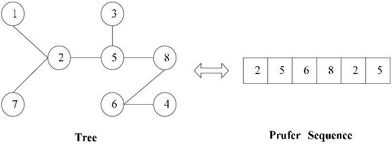
A Prüfer sequence or Prüfer code is a unique \(n\)-ary sequence (i.e. where \(a_i\in \set{1, \dots, n}\)) associated with a labelled tree with \(n\) vertices.

• The set of labelled trees with \(n\) vertices is isomorphic to the set of \(n\)-ary sequences of length \(n-2\).

Tree → Prüfer sequence: Find leaf \(s_1\in V(T)\) with the smallest label. The first term of the Prüfer sequence \(A\) will be the neighbour of \(s_1\). Delete \(s_1\) from \(T\) (i.e. iterate \(T=T\setminus \set{s_1}\)). Repeat this process until no vertices remain.

Prüfer sequence → tree: for \(n\)-ary sequence \(A=(a_1, a_2, \dots, a_{n-2})\), we construct the corresponding tree by finding the smallest \(a_0 \in \set{1, \dots, n}\) that is not in \(A\). We join vertex with label \(a_0\) to the first vertex in \(A\) (initially \(a_1\)). Next, we update \(A\) by removing the first element and appending \(a_0\) to the back end. This repeats until we have completely replaced \(a\); the last edge the two nodes missing from the last state of \(A\).

• A walkthrough is available here

Spanning Trees

We define \(\tau(G)\) as the number of spanning trees of connected, labelled graph \(G\).

• ADV we define \(\mathcal{T}(G)\) as the set of all spanning trees of \(G\)

• E.g. For a graph with adjacency matrix \(A_G=\begin{bmatrix}0&1&0&1 \\ 1&0&2&1 \\ 0&2&0&1 \\ 1&1&1&0 \end{bmatrix}\), we have \(D_G=\begin{bmatrix}2&0&0&0 \\ 0&4&0&0 \\ 0&0&3&0 \\ 0&0&0&3 \end{bmatrix}\), so \(A_G - D_G=\begin{bmatrix} 2&-1&0&-1 \\ -1&4&-2&-1 \\ 0&-2&3&-1 \\ -1&-1&-1&3 \end{bmatrix}\). If we take cofactor \(2, 2\), we evaluate \((-1)^{2+2} \det{\begin{bmatrix} 2&0&-1 \\ 0&3&-1 \\ -1&-1&3 \end{bmatrix}}=\dots=13\), which is the number of spanning trees in \(G\).

If all spanning trees in graph \(G\) pass through vertex \(v\in V(G)\) (i.e. \(v\) is a cut-vertex), then for the components \(C_1, C_2\) of \(G\) induced by \(v\), we have \(\tau(G)=\tau(C_1\cup\set{v})\times \tau(C_2\cup\set{v})\). This is because each component has a spanning tree that includes \(v\).

Bipartite Graphs

As pre-corollaries, we have \(\tau(K_{2, n})=n2^{n-1}\) and \(\tau(K_{3, n})=n^{2} 3^{n-1}\).

• Simplified explanation of \(\tau(K_{2, n})=n2^{n-1}\): there are \(n\) choices for the path that joins the \(2\) vertices on the "\(2\) side" through a vertex on the \(n\) side. Then, the remaining \(n-2\) vertices on the \(n\) side have \(2\) choices on the \(2\) side. So, by the multiplication principle, there are \(n2^{n-1}\) possible spanning trees.
• Simplified explanation of \(\tau(K_{3, n})=n^{2} 3^{n-1}\): we have \(2\) methods of joining the \(3\) side: either they are all a tree from one vertex on the \(n\) side, for which there are \(n\) choices, or they are connected by \(2\) different trees (forming a path), for which there are \(\displaystyle{n\choose 2}\) choices. Since these are separate rules, we use the sum rule to find \(\tau(K_{3, n})=n 3^{n-1}+\displaystyle{n\choose 2}\times 3! \times 3^{n-2}=n^{2}3^{n-1}\).

• Proof: Follows from Kirchoff's theorem and the cofactor expansion definition of the determinant (full proof in course notes)
• Aside: this could also likely be proved by generalizing the pattern from the \(m=2\) and \(m=3\) or by induction on \(m\).

ADV Non-labelled Trees

Enumerating non-labelled trees is a much less trivial problem, requiring knowledge of combinatorics not assumed or covered in this course.

• Quora: Does a formula for non-isomorphic trees on n vertices exist?
• OEIS: sequence of numbers of non-isomorphic trees on n vertices: \(1, 1, 1, 2, 3, 6, 11, 23, 47, 106\)

A useful way to manually generate all the non-isomorphic trees on \(n\) vertices is to list all trees \(T\) by \(\Delta(T)\), where \(\Delta(T)=k\) for each \(2 \geq k \geq n-1\). \(k=2\) corresponds to the graph \(P_n\) and \(k=n-1\) corresponds to the tree of depth \(2\) (i.e. \(W_{n}\setminus E(C_{n-1})\)).

ADV Relating Edge, Vertex, and Component Counts

Define the attributes of \(G\) as \(\#V(G)=n\), \(\#E(G)=m\), and \(c(G)=c\).

[!Theorem 7.5] ADV Theorem 7.5 For all graphs \(G\) we have \(m\geq n-c\), where \(m=n-c\) if and only if \(G\) is a forest.

• Proof: \(\impliedby\): Clearly, each component in the forest is a tree, and each component with \(c_i\) nodes needs exactly \(c_i-1\) edges. \(\displaystyle\sum\limits_{i=1}^{c} c_i=n\), since each node must be in a component, so it follows that \(\displaystyle\sum\limits_{i=1}^{c} (c_i-1)=\displaystyle\sum\limits_{i=1}^{c} c_i -\displaystyle\sum\limits_{i=1}^{c} 1=n-c\). \(\implies\): Having a cycle would definitionally require more edges, so if the equality holds, \(G\) must be a forrest.

• Proof: we take \(c=1\) and apply theorem 7.5

Minimum Connector Problem and Kruskal's Algorithm

Minimum Connector Problem: given a edge-weighted, (not necessarily connected) graph \(G\), what is the least expensive spanning tree? This problem can be solved with Kruskal's Algorithm (\(\Theta(E\log{E})\)).

• Proof: Clearly the algorithm terminates once \(n-1\) edges have been selected, which by definition won't form a spanning tree since edges are picked such that cycles are not formed. Since the edges of minimum weight are picked each time, this is the spanning tree of smallest weight.
• Aside: Kruskal's algorithm is a greedy algorithm.
• Aside: Kruskal's algorithm provides a lower bound on the travelling salesman problem

Interesting Conjectures

ADV Search Trees

A search tree augments a spanning tree with extra information that improves navigation within the graph: a root vertex \(\star{v}\), a parent function \(\text{pr} : V(T)\to V(T)\cup\set{\text{null}}\), and a level function \(\ell : V(T)\to \mathbb{N}\).

A search tree can be generated by starting with a random root node and randomly picking edges in the boundary that connect to that node, assigning the root as a parent, and repeating the process recursively:

• The structure of the search tree \(T\) is defined by \(V(T)=W\) and \(E(T)=F\).

Create-Search-Tree (Graph G, Vertex v* \in V(G)) -> pr (function), l (function):
    let W = {v*}
    let F = {}
    let pr(v) = null
    let l(v) = 0
    let Boundary = d(W)
    
    while(Boundary is nonempty)
        pick Edge e=xy with x in W and y not in W
        W = W \union {y}
        F = F \union {e}
        pr(y) = x
        l(y) = 1+l(x)
        Boundary = d(W)
    
    return functions pr, l 

Chapter 4 - Planarity

Definitions (4.1)

A planar graph is a graph that has a plane drawing/planar embedding, i.e. that can be drawn on a plane without any edges crossing.

• Many real-world situations modelled by graphs are planar, e.g. geographic maps

The crossing number \(\text{cr}(G)\) of graph \(G\) is the minimum number of crossings required to draw \(G\) in the plane.

• If \(G\) is planar, then \(\text{cr}(G)=0\).
• Proving a crossing number requires drawing the graph with that number of crossings, then proving one with less crossings cannot exist
• Turán conjecture: \(\displaystyle\text{cr}(K_{m, n})=\left\lfloor\dfrac{m}{2}\right\rfloor\left\lfloor\dfrac{m-1}{2}\right\rfloor\left\lfloor\dfrac{n}{2}\right\rfloor\left\lfloor\dfrac{n-2}{2}\right\rfloor\) (shown up to \(K_{7, 9}\))
• The crossing number problem is NP-complete

Characterizing Planar Graphs

• Proof of \(K_{3, 3}\): \(K_{3, 3}\) has a cycle of length \(6\), (and \(6\) vertices) so any plane drawing will consist this \(6\)-cycle and edges that are either completely inside or outside of this cycle (since otherwise a crossing would occur). There are three instances of these chords dividing the cycle in half; clearly at most one can go across the cycle and one outside. Adding the third one creates a crossing. So \(K_{3, 3}\) is not planar.
  • A similar argument can be made for \(K_5\) with a cycle of length \(5\).
• Strategy for proving non-planarity: find the largest cycle in the graph (i.e. one that contains all the vertices if possible), characterize the rest of the edges as fully "inside" or "outside" the cycle, then show these chords need to cross.

Two graphs are homeomorphic if one can be constructed from the other by "splitting" existing edges by inserting new vertices.

• We describe this process as the subdivision of an edge

• Proof: complicated af and not covered here

A good strategy for figuring out if small-ish graph are planar (i.e. have a subgraph homeomorphic to \(K_5\) or \(K_{3, 3}\)) is to draw vertices (and appropriate edges) one-by-one, taking care not to cross edges. Either a new vertex can be drawn without creating a crossing, or some subgraph homeomorphic to \(K_5\) or \(K_{3, 3}\) exists and can be identified by inspection.

Euler's Formula (4.2)

A planar graph \(G\) divides the plane into faces, including the unbounded infinite face "around" the graph.

• Proof: We use induction on \(m\). Base case: \(m=0\) clearly holds since the only connected graph has \(n=1\). Inductive case: assume formula holds for \(m=k\). Let \(G\) be a planar graph with \(k+1\) edges. If \(G\) is a tree, no new face was created (since no cycles were created), so an extra vertex must have been added; \((n-1)-m=n-(m+1)\), so the induction step holds. Otherwise, a cycle was created, so although the number of nodes \(n\) didn't increase, the number of faces increased by \(1\), so the sum still stays constant.

• We can use this to prove the non-planarity of \(K_5\) (point \(1\)) and \(K_{3,3}\) (point \(2\))

• Proof (covers that of Corollary 4.2.2): Since \(G\) has girth \(g\), by the faceshaking lemma, we have \(2m\geq gf\), where \(f=\# F(G)\), implying \(\frac{2}{g}e\geq f\). Subbing this into Euler's formula, we get \(v-m+\frac{2}{g}\geq 2\implies v+(\frac{2}{g}-1)m\geq 2\), from which we derive Corollary 4.2.2 through algebra.

• Proof: Assume for contradiction a simple planar graph exists where each vertex has degree of at least \(6\). Then, this graph has at least \(\frac{6n}{2}=3n\) edges. However, since \(G\) is planar, we much have \(m\leq 3n-6\), so we have \(3n \geq m \geq 3n-6\), which is impossible.

• Proof sketch: we use induction as before, but add an extra case where the additional edge connects two components together. This doesn't add a face or vertex, but decreases the number of components by \(1\), balancing the formula.

ADV Faceshaking Lemma

The footprint \(\text{fp}(H)\subseteq \mathbb{R}^2\) of subgraph \(H\) of \(G\) with planar embedding \((\mathcal{P}, \Gamma)\) is the union of the points and curves representing the vertices and edges in \(H\) when "rendered" in \(\mathbb{R}^2\).

• With this definition, we can recharacterize a face of \((\mathcal{P}, \Gamma)\) as a connected component of \(\mathbb{R}^{2}\setminus (\mathcal{P}, \Gamma)\), i.e. the complementary component of \((\mathcal{P}, \Gamma)\)

The boundary \(\partial F\) of face \(F\) is the set of edges and vertices whose curves and points (respectively) are contained in \(F\subseteq \mathbb{R}^2\).

The degree of face \(F\) is the sum of the number of edges and bridges adjacent to \(F\)

• A bridge across face \(F\) is an edge that is "inside" \(F\), but doesn't separate it, i.e. a peninsula or an edge crossing the infinite face.

• This follows from the duality between faces and vertices discussed later

Graphs on Non-planar Surfaces (4.3)

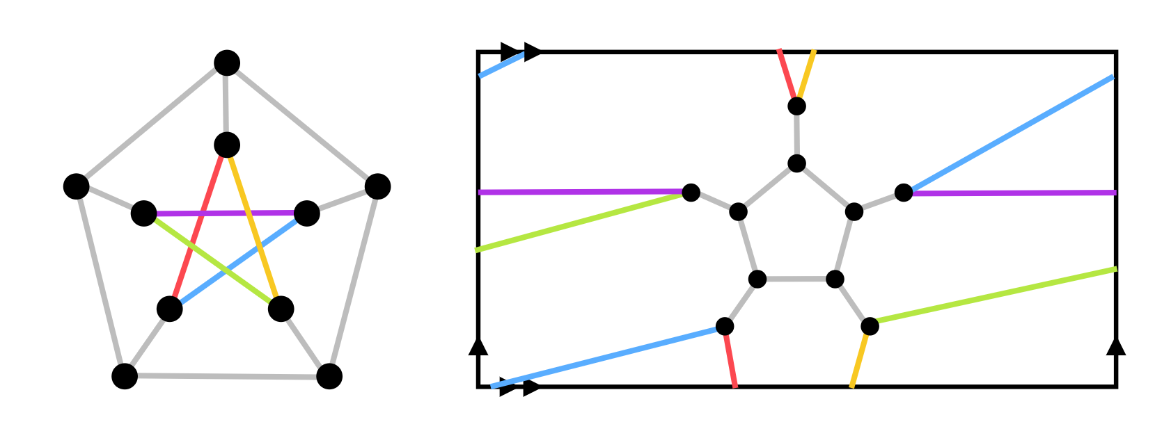
• E.g. Any graph \(G\) such that \(\text{cr}(G)=1\) (e.g. the Petersen graph) can be drawn on a torus without edge crossing; intuitively, we can wrap the crossing edge around the other side of the torus.

The genus \(g(G)\) of graph \(G\) is the smallest genus such that \(G\) can be drawn on a surface of that genus without crossings.

• In topology, a surface of genus \(g\) is topologically homeomorphic to a sphere with \(g\) handles.

• Proof: We draw \(G\) on a (genus \(0\)) plane with \(\text{cr}(G)\) crossings. Then, we construct a handle at each crossing and draw one edge over it and the other under it. Therefore, at most \(\text{cr}(G)\) handles are needed, meaning \(g(G)\leq\text{cr}(G)\)
• For most graphs, the inequality is strict, i.e. \(g(G)<\text{cr}(G)\) because multiple crossings can be planarly rerouted around handles

• Proof: much like our relation on the edge and vertex counts, the girth of at least \(3\) implied by "simple graph" implies \(3f\leq 2m\), which can be substituted into Euler's (genus-generalized) formula to find \(6-6g-3n+3m\geq 2m\), which is equivalent to the Theorem 4.3.3 since \(g\) must be an integer.

• Explanation: since \(K_n\) has \(\displaystyle{n\choose 2}=\dfrac{n(n-1)}{2}\) edges, we can substitute this into theorem 4.3.3 to find \(g(K_n)\geq\left\lceil\dfrac{(n-3)(n-4)}{12}\right\rceil\). Proving that this is an equality is much more difficult.

where the equality holds if and only if each face has degree \(3\), i.e. is a triangle.

• Proof: by the handshaking lemma, we have \(\displaystyle\sum\limits_{d=1}^{\infty}d n_d = \sum\limits_{v\in V}\text{deg}(v)=2\times \# E(G)\), since all but finitely many terms in the infinite series will be \(0\). By the faceshaking lemma, \(2\times \# E(G) = \displaystyle\sum\limits_{f\in \mathcal{F}}\deg{F}\geq 3\times \# \mathcal{F}\). Since \(G\) is connected, by Euler's formula, we have \(\# V - \# E + \# \mathcal{F}=2\). Together, this yields \(12=\displaystyle 6\sum\limits_{d=1}^{\infty}n_d - \sum\limits_{d=1}^{\infty}d_n =\sum\limits_{d=1}^{\infty}(6-d)n_d\), implying the proposition.

ADV Stereographic Projection

Stereographic projection is the process of extending the line segment that intersects the center of a sphere and a point on the surface until it intersects with a plane (\(\mathbb{R}^2\)) below the sphere. A graph that is planar on a sphere can be stenographically projected onto a flat plain while retaining its planarity, and vice-versa.

• The "northern hemisphere" of the sphere is projected "up into infinity", so we cannot draw vertices on it. This forms the face at infinity, which is the "outside" face of a planar embedding.
• This suggests that all convex polyhedral graphs are planar

Thus, the plane is topologically homeomorphic to the sphere; a graph has a planar embedding if and only it can be drawn on a sphere without crossings.

Duality (4.4)

The dual graph \(\star{G}\) of planar graph \(G\) is the graph obtained by drawing a vertex in each face of \(G\) and connecting the vertices of adjacent faces with edges.

• Since each edge in \(G\) separates two faces by definition, we simply cross each edge in \(G\) with another edge in \(\star{G}\)
• E.g. the dual of a Voronoi Diagram is a Delaunay Triangulation
• Two isomorphic graphs may have non-isomorphic duals, i.e. duality isn't well defined over isomorphism

If \(G\) is a connected planar graph, then \(\star{G}\) will also be a connected planar graph.

• Proof: By the definition of \(\star{G}\), clearly it will have \(f\) vertices and \(m\) edges (this remains unchanged). We find that \(\star{G}\) has \(n\) faces from Euler's formula.
• So, for any choices of point within a face of the graph, a planar embedding must exist where those points form the endpoints of the curves connecting the vertices of the dual graph (more in Lemma 8.27 in the 249 notes).

• Proof:

Dual Concepts

Properties are dual if property \(\mathsf{A}\) of \(G\) corresponds to property \(\mathsf{B}\) of \(\star{G}\). Thus, theorems about \(\mathsf{A}\) in \(G\) correspond to theorems about \(\mathsf{B}\) in \(\star G\).

• Faces and vertices are dual objects
• Cycles and cutsets are dual objects
  • So, \(\text{girth}(G)=\lambda(\star{G})\) and vice versa
• Bridges and Loops are dual concepts
  • I.e. for planar graph, a bridge is a "peninsula" jutting into a face
• Having an Eulerian cycle and being bipartite are dual concepts.
  • Proof sketch: Eulerian cycle in \(G\) \(\implies\) each degree of \(G\) is even \(\implies\) (dual) each face of \(\star{G}\) as an even degree \(\implies\) \(\star{G}\) has no odd cycles \(\implies\) \(\star{G}\) is bipartite.

• Proof (half): \(\implies\): If \(C\) is a cycle in \(G\), then it encloses at least one face of \(G\). Thus, the corresponding faces in will enclose a vertex in \(\star{G}\). So, the set of edges in \(\star{G}\) that "cross" the edges of \(C\) in \(G\) clearly disconnect the enclosed vertex in \(\star{G}\) from the rest of the graph. \(\impliedby\): similar proof.

ADV Appendix: Extra Concepts

Platonic Solids

A platonic solid is any polyhedron represented by a connected \(d\)-regular plane embedding that is face-\(k\)-regular. There are exactly \(5\) such graphs (where embedding is unique up to isomorphism), i.e. possible values of \((d, k)\):

• Tetrahedron (\(K_4\)): \((3, 3)\)
• Octahedron: \((4, 3)\)
• Cube (\(Q_3\)): \((3, 4)\)
• Icosahedron: \((5, 3)\)
• Dodecahedron: \((3, 5)\)

Deriving Global Statements about Types Planar Graphs

Often, if we know properties about a graph \(G\), we can describe \(V(G)\), \(E(G)\), and \(F(G)\) (if \(G\) is planar) as series/sums, usually utilizing the handshaking and faceshaking lemmas. We can then substitute these into Euler's formula to relate them in a sequence.

• E.g. for simple, cubic, bridgeless, planar graphs, if \(F_d\) is the number of faces of degree \(d\), we find the identity \(3F_3+2F_4 + F_5 (+ 0F_6) - F_7 - 2F_8 - 3F_9-\dots=12\)

We can then use this formula to find properties about the type of graph we've described.

• E.g. for simple, cubic, bridgeless, planar graphs, (with the sequence above) we find that if the faces consist entirely of pentagons, then there must be exactly \(12\) faces (i.e. the dodecahedron). We also find that if the graph consists entirely of rectangular faces, it must have exactly \(6\) faces (i.e. the cube). This sequence in particular can be used to prove useful faces about the uniqueness of the platonic solids (with the exception of the icosahedron, which is not cubic).

Chapter 5 - Coloring

Coloring Vertices (5.1)

Loopless graph \(G\) is \(k\)-colorable if we can color the vertices of \(G\) with \(k\)-different colors such that no adjacent vertices are the same color.

• A proper \(k\)-coloring of graph \(G\) is a function \(f:V\to K=\set{1, 2, \dots k}\) that assigns each vertex of \(G\) a color (\(\in K\)) such that \(vw\in E(G) \implies f(v)\ne f(w)\).
• \(k\)-partition and \(k\)-colorability are the same thing, e.g. bipartite \(\iff\) \(2\)-colorable

The chromatic number \(\chi (G)\) of \(G\) is the integer \(k\in \mathbb{N}\) such that \(G\) is \(k\)-colorable but not \(k+1\)-colorable.

• Proof: clearly, any clique of size \(k\) has chromatic number of at least \(k\), since the clique is a complete subgraph of size \(k\). There are additional non-clique ways to increase this number, explaining why this theorem isn't an equality.

• Proof by induction on \(n\): Base case: for \(n=1\), the only simple graph is \(N_1\). Clearly, \(\chi(N_1)=1\leq \Delta(N_1)+1=0+1=1\). Induction hypothesis: Assume \(\chi(G)\leq \Delta(G)+1\) holds for a graph \(G\) with \(k\) vertices. Let \(G'\) have \(k+1\) vertices, and choose any vertex \(v\) and consider \(G'\setminus\set{v}\). By the induction assumption, this must be \(\Delta(G')+1\)-colorable. \(v\) had a most \(\Delta(G)\) neighbours, so we can color it a different color than all of these; so \(G'\) must be \(\Delta(G')+1\) colorable, completing the induction hypothesis.

• Remark: this algorithm is not optimal (i.e. it doesn't find the least coloring (and thus chromatic number) of the graph), but it can be used to place a bound on the chromatic number of a graph.
• There is always a way to choose the order of \(G\)'s vertices such that this algorithm only uses \(\chi(G)\) colors. However, we don't know this order, and being able to find it is basically the whole problem anyway

Aside: An open problem in graph theory is the chromatic number of the unit distance graph of \(\mathbb{R}^2\), i.e. the graph where the vertices are the points of \(\mathbb{R}^2\) and vertices are adjacent iff they have a Euclidean distance of \(1\). Currently, we know this number is between \(5\) and \(7\) (inclusive).

Coloring Vertices of Planar Graphs

Note: these theorems are equivalent to finding the minimum number of colors needed to color the faces of a cubic planar graph without bridges. If graph can be face-colored with \(k\) colors, it is \(k\)-colorable(f).

• Proof: we proceed by induction on \(n\). Base case: for \(n=1\), \(N_1\) is definitely \(6\)-colourable. Inductive case: assume a simple planar graph with \(k\) vertices is \(6\)-colorable. If \(G'\) is a simple planar graph with \(k+1\) vertices, it must have a vertex \(v\) of degree at most \(5\) (since it is planar). So, \(G' \setminus\set{v}\) will be \(6\)-colorable by the induction assumption. Thus, we can "add \(v\) back" and color differently than its (at most \(5\)) neighbours. So, \(G'\) is also \(6\)-colorable, completing the inductive proof.

• Proof: we proceed by strong induction on \(n\). Base case: again, \(N_1\) is clearly \(5\)-colorable. Assume any graph \(G\) with \(k\) vertices or less is \(5\)-colorable. Again, since \(G\) is a simple planar graph, it has a vertex \(v\) of degree at most \(5\). By the induction assumption, \(G\setminus\set{v}\) is \(5\)-colorable. If the neighbours of \(v\) aren't all different colors, clearly we can pick a color for \(v\), so \(G\) is trivially \(5\)-colorable in this case. If each neighbour is a different color, there must be at one pair \(v_i, v_j\) of these neighbours that aren't adjacent, since otherwise \(G\) would contain a \(K_5\) subgraph and thus not be planar. If we contract edges \(v_i v\) and \(v_j v\), we obtain a graph with \(k-1\) vertices that can be \(5\)-colored by the induction hypothesis. So, we can replace \(v_i v\) and \(v_j v\), assigning them the same color. \(v\) now has \(5\) neighbours with \(4\) colors, so we can color \(v\) the fifth color.

• Corollary: every cubic planar graph with no bridges is \(4\)-colorable
• Proof: lol

Remark: since planar graphs always have a well-defined dual, coloring theorems also apply to the dual structures as well, e.g. \(4\)-colorability is equivalent to \(4\)-colorability(f).

Remark: many planar coloring proofs involve induction or strong induction on the number of vertices, where some graph \(G\setminus\set{v}\) is used to apply the induction hypothesis.

ADV Chromatic Number and Girth

Generally, a large chromatic number implies a high level of interconnection between vertices, while large girth suggests the opposite. However, graphs with arbitrarily large (though not strictly arbitrary) girth and chromatic number can be found.

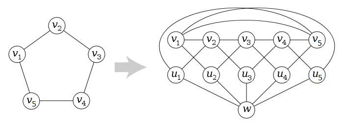
We define the Mycielski construction of graph \(G\) as follows: let \(V'=\set{v' : v\in V(G)}\) be a set of "new" vertices disjoint from \(V(G)\), and \(z\) be another vertex not in \(V(G) \cup V'\). Let Mycielski construction \(\mathcal{M}(G)\) of \(G\) be the graph with vertices \(V(\mathcal{M}(G))=V(G)\cup V' \cup \set{z}\) and edges \(E(\mathcal{M}(G))=E(G)\cup\set{zv' : v\in V(G)}\cup\set{v'w : v\in V \text{ and } vw \in E(G)}\).

• \(\mathcal{M}(G)\) will contain \(G\) as a subgraph

• By corollary, for any \(k\geq 2\) there exists a \(k\)-chromatic graph of girth \(4\). We find that examples for \(k=2, 3\) are easy to find, and iterating \(\mathcal{M}(C_5), \mathcal{M}( \mathcal{M}(C_5)), \dots\) settle the remaining cases.
• Both of the above theorems may be proven as exercises

Perfect Graphs (5.2)

A perfect graph is a simple graph where every induced subgraph \(H\subseteq V(G)\) of \(G\) satisfies \(\chi(H)=\omega(H)\), i.e. for every subgraph, the chromatic number is the size of the largest clique in the subgraph.

• Any \(K_n\), bipartite graphs, and (thus) trees are perfect
• \(C_n\) is perfect for even \(n\) or \(n=3\)

An odd hole in graph \(G\) is an induced cycle of odd length with no chords. The complement of an odd hole is an odd antihole (i.e. if the odd hole is \(C_{2n+1}\), then an odd antihole is \(C_{n2+1}\setminus K_{2n+1}\))

Note: in perfect graphs, the graph coloring and maximal clique problems are of class \(P\).

Edge Coloring (5.3)

A graph \(G\) is \(k\)-colorable(e) if its edges can be colored with \(k\) colors such that no adjacent edges are given the same color. \(G\) has chromatic index \(k\), denoted \(\chi'(G)=k\) iff it is \(k\)-colorable(e) but not \(k=1\)-colorable(e).

Vizing's Theorem implies loopless cubic graphs either have \(\chi'(G)=3\) or \(\chi'(G)=4\). A snark is a simple bridgeless cubic graph with chromatic number \(\chi'(G)=4\), e.g. Petersen's graph.

• Proof:
  • Odd \(n\): We can \(n\)-color(e) \(K_n\) by arranging the vertices as a regular \(n\)-gon and coloring each edge of the \(n\)-gon cycle a different color. Then, each edge in the rest of the graph is colored like the edge in the \(n\)-gon cycle that it is parallel to. We know \(K_n\) cannot be \(n-1\)-colorable because we could color at most \(\dfrac{(n-1)(n-1)}{2}\) edges; \(K_n\) has \(\dfrac{n(n-1)}{2}\geq \dfrac{(n-1)(n-1)}{2}\) edges.
  • Even \(n\): We \(n\)-color(e) \(K_{n-1}\) as described above, then add one additional vertex and connect it to each existing one. Because each vertex in \(K_{n-1}\) has degree \(n-2\), there will be one (unique) color left over from each vertex in \(K_{n-1}\).
• Aside: this mimics the structure of \(A_2(n, d)=A_2(n-1, d-1)\) for even \(n\) in coding theory

Snarky Theorems

• Proof: A cubic graph must have an even number of vertices, so the hamiltonian cycle has an even amount of edges, meaning it can be \(2\)-colored(e). The rest of the edges are chords inside this cycle; since the graph is cubic, no vertex is connected to more than one chord, so the rest of the (chords) (edges) can be colored with one color.

• This is equivalent to the four-color theorem; we can assign colors to edges based on the colors of the faces that the edges separate. Namely, if a planar graph is \(4\)-colored(f), each disjoint pair of face color combinations that an edge can separate is assigned a color. There are \(\displaystyle{4\choose 2}=6\) such combinations, so there are \(3\) mutually disjoint pairs. These three colors correspond to the \(3\)-coloring(e) of the simple bridgeless planar cubic graph.

• If Tait's conjecture were true, we could prove the four-color theorem by showing \(G\) is a cubic planar graph with no bridges \(\implies\) \(G\) is Hamiltonian (by Tait's conjecture) \(\implies\) \(G\) is \(3\)-colorable(e) \(\implies\) \(G\) is \(4\)-colorable(f).

• Proof: We proceed by induction on the number of edges
  • Base case: For \(m=0\) and \(m=1\), the graphs \(N_1\) and \(P_2\) (respectively) satisfy \(\chi'(G)=\Delta(G)\).
  • Inductive case: Assume any bipartite graph \(G\) with \(k\) edges satisfies \(\chi'(G)=\Delta(G)\). Let \(G'\) be a bipartite graph with \(k+1\) edges. For an edge \((uv)=e\in E(G')\), \(G'\setminus\set{e}\) can be colored(e) using \(\Delta(G)\) colors. In \(G'\setminus\set{e}\), clearly \(\deg{u}, \deg{v}\leq \Delta(G)-1\), so \(u\) and \(v\) are both missing a color; we will denote them \(\alpha\) and \(\beta\) respectively. Clearly, if \(\alpha=\beta\), then we assign \(e\) color \(\alpha\). If \(\alpha\ne \beta\), we consider the \(\alpha/\beta\) Kempe chains (chains of two alternating colors) from each \(u\) and \(v\). \(G'\) is bipartite, so it cannot have an odd cycle; thus the chains cannot link. Thus, we can swap \(\alpha\) and \(\beta\) on the chain from \(v\), then assign \(e\) color \(\beta\).

By corollary, \(\chi'(K_{r, s})=\max\set{r, s}\).

Chromatic Polynomials (5.4)

For a simple labelled graph \(G\in\mathcal{G}_n\), we define the chromatic function/chromatic polynomial \(P_G(k)\) of \(G\) as, for each \(k\in \mathbb{N}\), the number of ways to \(k\)-color the vertices of \(G\) such that no two adjacent vertices are the same.

• \(P_G(k)\) is always a polynomial of degree \(n\)
• If \(\chi(G)=k\), then \(P_G(\ell)=0\) for \(\ell<k\)
• Certain coefficients always have the same value
  • \(k^n\) term: \(1\)
  • \(k^{n-1}\) term: \(- \#E(G)\)
  • \(k^0\) (constant term): \(0\)
  • Aside: these seem to mimic the meanings of terms in the characteristic polynomial of a matrix. Is this related to spectral theory?
• Coefficients alternate in sign
• If \(G\) is a simple planar graph, then \(P_G (4)>0\)

• So, we get the definition for the contracted edge graph \(P_{G/\set{e}}(k)=P_{G\setminus\set{e}}(k)-P_G(k)\)
• We use \(G-\set{e}\) to denote deletion so it's easier to distinguish from contraction
• Proof sketch: if edge \(e=uv\), then in \(G-\set{e}\), \(u\) and \(v\) may be colored differently or the same color. In \(G/ \set{e}\), \(u\) and \(v\) "become the same vertex", meaning they must be colored the same. So, for any \(k\), the number of ways to color \(u\) and \(v\) differently (which is required in \(G\)) is the total number of ways to color them (like in \(G-\set{e}\)) minus the number of ways to color them the same color (like in \(G/\set{e}\)).

Aside: how are chromatic polynomials connected with generating series? Are they an example of generating series?

Finding Chromatic Polynomials

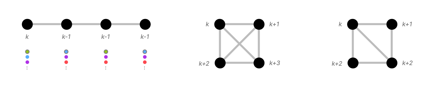
Generally, we find chromatic polynomials by determining how many colors can be used to color each vertex in a graph successively. For example, the first vertex we pick can be colored \(k\) ways; one adjacent to that can be colored \(k-1\) ways, and one adjacent to both can be colored \(k-2\) ways. Each time, we figure out how many ways the successive vertex can be colored. We can then find all the ways to color the vertices by multiplying these terms together (product rule).

• Since the polynomial has an argument for the number of colors, we also count starting with an arbitrary number of colors (\(k\)). The number of ways to color each vertex expressed as \(k-m\).
• In the above example, we found the chromatic polynomial of \(C_3\) is \(P_{C_3}=k(k-1)(k-2)\).
• Aside: how can we characterize which graphs' chromatic polynomials can be "read off" like this

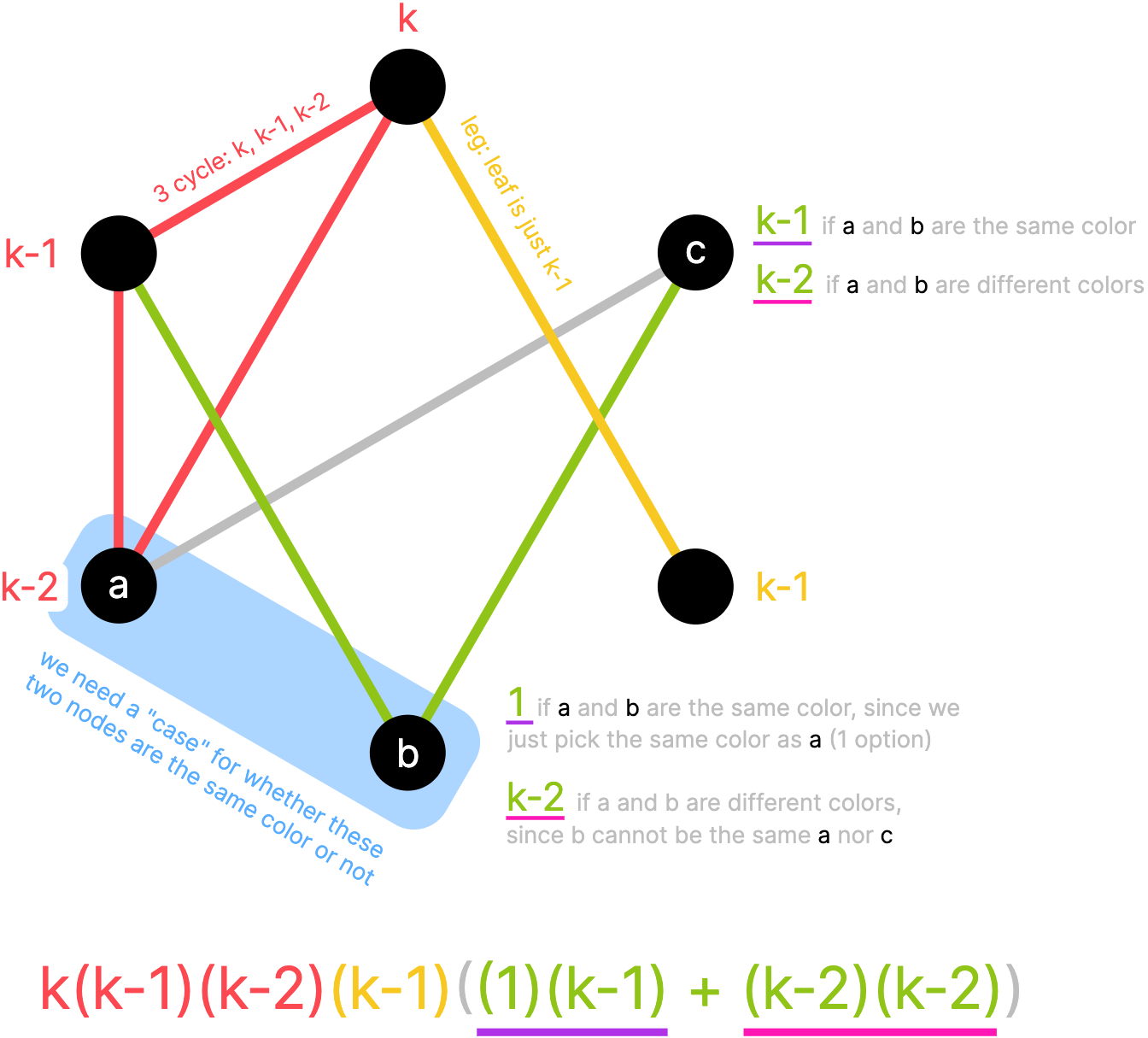
We can also divide colorings into disjoint cases, then add the different resulting polynomials together (sum rule). Usually, these cases are whether two (non-adjacent) vertices are the same or different colors.

Finally, we can use the decomposition theorem to express the chromatic polynomials of complex graphs as the differences between chromatic polynomials of simpler graphs.

• Specifically, holes should be decomposed.

Overall, finding chromatic polynomials is a combinatorial counting exercise, but we count down from an arbitrary \(k\) instead of up from \(1\). [The factored forms of] chromatic polynomials themselves are a way to capture the counting behaviour of enumerating graph colourings.

Example

Chromatic Polynomials of Common Graphs

Chapter 6 - Digraphs

Definitions and Elementary Theorems (6.1)

Digraphs

A directed graph or digraph \(G\) is a tuple \((V(G), A(G))\) where \(V(G)\) is a set of vertices and \(A(G)\) is a set of directed arcs that connect the vertices. An arc connecting vertices \(v, w\in V(G)\) is denoted \(vw\) (not equivalent to \(wv\))

• Essentially, a digraph is a like a graph, but edges have direction
• Most of our definitions extend naturally to digraphs
• Aside: we can treat a "regular" graph like a digraph where each edge is a pair of oppositely directed arcs

The out-degree \(\text{outdeg}(v)\) of vertex \(v\) in digraph \(G\) is the number of arcs leaving \(v\); the in-degree \(\text{indeg}(v)\) of \(v\) is the number of arcs that end in \(v\).

A simple digraph is a loopless digraph with unique arcs (again, \(wv\ne vw\))

The underlying graph of digraph \(G\) is the "regular" graph obtained by replacing each arc with an edge

• Aside: we can consider the underlying graphs as equivalence classes over directed graphs \(G/\sim\), where arcs \(a\sim b\) if they connect the same vertices (not necessarily in the same order).

Connectivity

A digraph \(G\) is strongly connected if a (directional) path exists between any two vertices in \(G\).

• This is an extension of the regular definition for digraphs

A vertex \(v\in V(G)\) in digraph \(G\) is a source if \(\text{indeg}(v)=0\), i.e. all adjacent arcs point away from \(v\); \(v\) is a sink if \(\text{outdeg}(v)=0\), i.e. all adjacent arcs point towards \(v\).

• A strongly connected digraph cannot have a source, nor can it have a sink
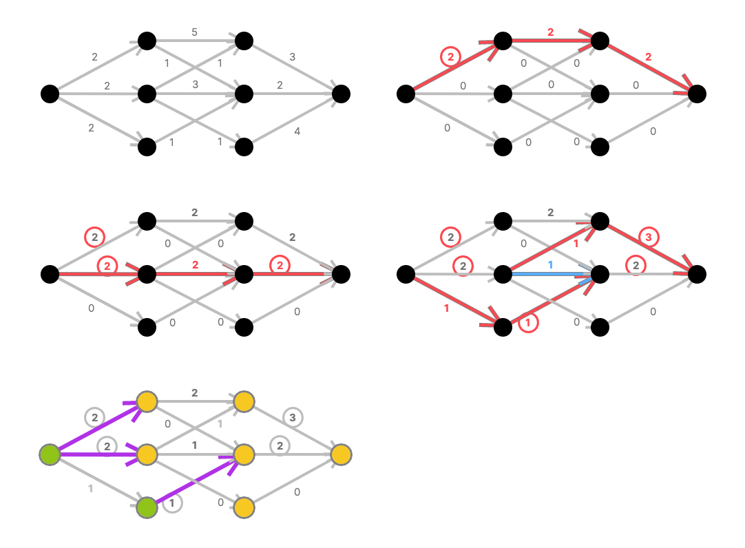
• Aside: Enumerating source → sink paths can be done with a recurrence relation, so finding every source-sink path (and thus the critical path) can be done with dynamic programming.

Eulerian and Hamiltonian Digraphs (6.2)

Eulerian and Semi-Eulerian Digraphs

• Proof: Pick an arbitrary vertex \(v_0\), then pick an arbitrary outgoing arc from \(v_0\) to some \(v_1\). Continue this process. At some point, you must reach a vertex that is in the sequence \(v_0\to v_1\to v_2 \to \dots\). This forms a cycle.

• Proof: \(\implies\) is clear via the same reasoning as the undirected case. \(\impliedby\) like in the undirected case, we proceed by strong induction with base cases \(N_1\) and the graph with one vertex and one arc-loop. Like before, we can assume an eulerian cycle exists, remove it, assume by the induction hypothesis that an eulerian cycle exists in each component left behind, then move around the main cycle and follow the eulerian cycle around each component when it is reached.

Hamiltonian Paths and Tournaments

A tournament is a digraph where each pair of vertices is joined by exactly one arc. i.e. its underlying graph is a complete graph \(K_n\).

• Such graphs are named tournaments because if each vertex represents a team and all teams play each other, the direction of the arc between two teams can encode who won each match. This can "rank" players.

• UAlberta theorem!
• Proof (1): We proceed by induction. Base case: for \(n=2\), the directed path graph \(P_2\) is clearly semi-Hamiltonian. Inductive case: assume tournaments with \(k\) vertices are Hamiltonian or semi-Hamiltonian; let \(G\) have \(k+1\) vertices. Clearly, for arbitrary \(v\in V(G)\), \(G\setminus\set{v}\) is Hamiltonian or semi-Hamiltonian by the induction assumption. If \(G\setminus\set{v}\) is Hamiltonian, then clearly \(G\) is semi-Hamiltonian. Otherwise, let \(G\) by semi-Hamiltonian, with semi-Hamiltonian path \(v_1\to v_2\to v_3\to \dots \to v_k\). If edge \(vv_i\) is in \(G\), then \(v_1\to \dots \to v_{i-1}\to v \to v_{i+1} \to \dots\) is semi-Hamiltonian. Otherwise, if \(vv_i\) isn't in \(G\) for any \(i\leq k\), then edge \(v_i v\) must be in \(G\) (since it is a tournament), and thus \(v_1\to v_2 \to \dots \to v_k \to v\) is a semi-Hamiltonian path.
• Proof sketch (2): we can use induction to show that \(G\) has a cycle of length \(k\).

A tournament is transitive if arcs \(uv\) and \(vw\) imply arc \(uw\).

• Proof: \(\implies\): Clearly, for a cycle in the tournament of size \(n\), the first \(n-1\) arc form a path from \(v_1\) to \(v_{n-1}\). The last arc of the cycle isn't \(v_1 v_{n-1}\) since we already know it must be \(v_{n-1}v_1\), since it forms a cycle. So, the tournament isn't transitive. \(\impliedby\): if \(G\) has no cycles, it must be semi-hamiltonian with semi-hamiltonian path \(v_1\to v_2\to\dots\to v_n\). Clearly, every path must be in the form \(v_i v_j\) for \(i < j\), otherwise a cycle would exist. Therefore, any subpath of the semi-hamiltonian path is transitive; this includes all the vertices of the graph that are reachable, so the whole graph is transitive.

So, there are two types of tournaments: strongly connected ones with Hamiltonian paths, or transitive ones with semi-Hamiltonian paths and no cycles.

Critical Paths (6.3)

In task scheduling problems, some subtasks can be completed whenever while others must be completed in a particular order, i.e. after a specific subtask. Such problems can be expressed as arc-weighted digraphs, where arcs (weighted by time) represent subtasks and two arcs are adjacent if one must be complete before the other begins. Our goal is to minimize the time needed to complete all the subtasks; this is represented by the longest path from source to sink (critical path).

• This works because this longest path must be completed, and thus sets a lower bound on how long it might take to complete the task. It also indicates which tasks should be started immediately, and which can be waited on without increasing the time it takes to complete the task.

For critical path-finding algorithms, take an algorithms course!

Networks (6.4)

A network is a weighted digraph with one source and one sink. Each arc \(a\) is weighted by its capacity \(\psi(a)\) which defines the maximum unit (e.g. electric current, water, etc) that can travel through it at a given moment in time.

• The out-degree of each vertex \(v\) in network \(G\) is the sum of capacities leaving \(v\); the in-degree of \(v\) is the sum of capacities entering \(v\).

Definitions: Flows and Cuts

A flow \(\phi\) in network \(G\) is a function \(\phi : A(G)\to \mathbb{R}^{0+}\) that assigns each arc \(a\in A(G)\) a non-negative real value \(\phi (a)\) where:

• \(\phi(a)\leq \psi(a)\) for each arc \(a\in A(G)\)
• For all vertices \(v\in V(G)\), \(\text{indeg}(v)=\text{outdeg}(v)\) with the exception of the source and sink

So, informally, a flow describes a way that the unit can "flow" (ahaaaaaa) through the network without pooling or exceeding the capacity of any particular pathway.

• Aside: this is reminiscent of Kirchoff's laws for electric circuits. This is the same Kirchoff that proved the matrix-tree theorem in chapter 3…

The zero-flow \(\phi : A(G)\mapsto 0\) maps each arc to \(0\).

A saturated arc is an arc \(a\) such that \(\phi(a)=\psi(a)\)

The value of a flow is the sum of the flows out of the source and/or the sum of the flows into the sink. Clearly these must be equal by the handshaking dilemma; this also makes sense in our informal interpretation.

The maximum flow is a flow \(\phi\) that has the largest possible flow value for the network; we often want to find this \(\phi\) to optimize the network.

A cut \(C\subseteq A(G)\) in digraph \(G\) is a set of arcs whose removal disconnects the source from the sink. The cut's capacity is the sum of the capacities of the cut, i.e. \(\displaystyle\sum\limits_{a\in C}a\)

• Often, our goal is to find the minimum cut, i.e. the cut with the smallest capacity

Max-Flow Min-Cut Theorem

• This makes intuitive sense as a bound; clearly the minimum cut cannot be smaller than the maximum flow, or "too much unit" would be flowing through the subset of arcs defined by the cut at any moment in time

A flow-augmenting path in network \(G\) is a path where arcs can be travelled in either direction if

1. Each forward-travelled arc in the path is unsaturated
2. Each backward-travelled arc in the path has nonzero flow

So, if a path has a saturated arc when traveling forward or a zero-flow arc when travelling backward, then the path cannot be flow-augmented (and thus nor can the network?)

Flow-augmenting paths can be used to find maximum flows because they can be iteratively improved. Note that the "path" itself isn't always being changed, but the amount traveling through each arc in the path is tweaked.

The minimum cut is derived from the maximum flow in network \(G\) by bipartitioning it into \(V, W\subseteq V(G)\), where \(V\) contains the source and any vertices that can be reached from it by flow-augmenting paths and \(W\) contains all other vertices. The arcs joining vertices in \(V\) to those in \(W\) (i.e. \(\partial V=\partial W\)) form the minimum cut.

The maximum flow \(\phi\) of network \(G\) can be thought of as a union/sum of a subset of the source to sink paths in \(G\) such that the capacity of each arc isn't surpassed. This subset may not be (and usually isn't) unique.

Finding Max Flows/Min Cuts

Generally, I find the best way to find maximum flow in a network is to do a depth-first search of all the source → sink paths in the network. Each time, I find the smallest slack left in a single arc in the path, and increase the flow through each of the arcs by that slack. Eventually, there will clearly be no way to leave the sink/get to the source; the max flow is thus found.

• Once a node is saturated (i.e. it has reached its maximal input/output), any paths leading to it don't need to be considered and can be crossed out
• As a matter of notation, arcs with \(0\) capacity are crossed out and the numbers denoting the flow through a saturated arc are circled
• As a sanity check, the input/output should match for each node
• Flow-augmenting paths can be found without travelling backwards; this adds complexity to the search and I find it easier not to use it

Minimum cut can be found with a recursive "choke point" algorithm. The arcs connecting directly to the sink form the initial cut (note that this is indeed a cutset). Then, consider the total weight of the arcs leading into the first arc. If they have less capacity than the arc itself, they replace that arc in the cutset.

• Note that this must be explored to full depth in both cases: even if the sum of capacities leading into a node is greater than its path to the sink, previous arcs even earlier in the network might have a smaller capacity.

ADV Appendix: Markov Chains

A Markov chain or chain is a network where every vertex has the same capacity (usually \(1\)), i.e. the capacities of the arcs leaving the node add up to \(1\).

The network encodes a system; the vertices encode states of the system and the arcs joining states represent the transition probabilities, i.e. the chance of moving from one given state to another at a particular timestep.

• An irreducible chain is strongly connected, i.e. every state can (eventually) be reached from any other state
• A chain is absorbing if it has an inescapable state, i.e. a state that points back to itself with probability \(1\).
• A transient state is a state that will never be visited after some other state is reached. Otherwise, the state is persistent.

A state \(E_i\) in a chain \(M\) is periodic with period \(t\) if it is only possible to return to \(E_i\) after a period of time that is a multiple of \(t\). Otherwise, \(M\) is aperiodic.

• So, vertex \(E_i\) is periodic iff every closed trail in the chain's associated digraph containing \(E_i\) has a length that is a multiple of \(t\).
• An ergodic state is both persistent an aperiodic

The transition matrix of a chain is the adjacency matrix of its digraph.

• The eigenvectors of this matrix encode the probabilities of a given state the "current" state at any timestep \(t\) for \(t \to \infty\). This property can be linked to Kirchoff's Theorem/Matrix Tree Theorem by considering the total set of possible timestep paths through a Markov chain as a tree (more information).

Chapter 7 - Matchings

Introduction to Matchings (7.1)

Matchings

A matching \(M\) in \(G\) is a subset \(M\subseteq E(G)\) of the edges of \(G\) where each vertex in the spanning subgraph \((V(G), M)\) of \(G\) has a degree of at most \(1\).

• A vertex \(v\in V(G)\) is \(M\)-saturated if it has degree \(1\) in \((V(G), M)\) and \(M\)-unsaturated if it has degree \(0\) in \((V(G), M)\)
• A perfect matching saturates every vertex in \(V(G)\).

The neighbourhood of \(S\subseteq V(G)\) on graph \(G\) is the set of edges in \(E(G)\) that have at least one endpoint in \(S\), i.e. \(N(S)=\set{v\in V(G) : vw\in E \text{ for some } w\in S}\). So, \(\text{neighbourhood}(S)=\partial S\cup \set{e\in E(G) : e \in \mathcal{P}(S)}\)

Hall's Marriage Theorem

Hall's Marriage Problem: Given bipartite graph \(G\) with bipartitions \(V\) and \(W\), does there exist a one-to-one correspondence (i.e. edges) between the vertices of \(V\) and some subset \(W_0\) of \(W\)?

• Proof sketch: \(\implies\): clearly, if a solution exists, then each subset of \(W\) of size \(k\) matches at least the \(k\) members of \(V\) given by the solution. If they didn't, there simply wouldn't be enough elements in \(V\) for the matching to occur. \(\impliedby\) can be proven by strong induction on the size of \(W\).

Contrapositive statement: if there exists a union of subsets \(W_0\subseteq W\) of size \(k\) that has less than \(k\) elements, then a full matching cannot exist.

• In this case, the largest different between the size union of some subsets and the number of subsets in that union is the number of vertices that will not be matched. Additionally, the vertices missing from any maximum matching will be in the union

Often, this is introduced as \(W\) being a set of girls and \(V\) being a set of boys, where vertices are adjacent across the bipartition of the girl and boy in question like each other. Then, the question becomes whether every girl can marry a boy she likes.

• The version of this problem that lets gay people out of the closet is more computationally difficult.

An alternate graph-theoretical statement of Hall's Marriage Theorem is as follows: Let \(G\) be bipartite with bipartition \((A, B)\). Then \(G\) has an \(A\)-saturating matching if and only if for all subsets \(S\subseteq A\), \(\# N(S)\geq \# S\), where \(N(S)\) is the neighbourhood of \(S\).

• This can be proven as an exercise

Combinatorial (Set) Formulation

Suppose we have a set of girls \(G=\set{g_1, g_2, \dots, g_m}\) and boys \(B=\set{b_1, b_2, \dots, b_n}\). Each girl knows a subset of the boys, i.e. \(g_1\) knows \(B_1\subseteq B\), \(g_2\) knows \(B_2\subseteq B\), etc. Is it possible to "match" each girl with a different boy, where the girl knows the boy in each "matching"?

For a finite, non-empty set \(B\) and family \(F=\set{B_1, B_2, \dots, B_n}\) where \(\varnothing\ne B_1, B_2, \dots, B_n \subseteq B\), a transversal of \(F\) is a set of \(n\) distinct elements of \(B\) such that exactly one element is chosen for each element \(B_n\in F\).

• Proof by this is just a thinly veiled restatement of Hall's marriage theorem

ADV Covers and König's Theorem

Covers

A cover \(C\) of graph \(G\) is a subset \(C\subseteq V(G)\) such that every edge in \(E(G)\) as at least one edge in \(C\), i.e. for all \(e\in E(G)\), \(e\cap C\ne \varnothing\) (were \(e=\set{a, b}\subseteq V(G)\times V(G)\)).

• A minimum cover \(C_0\) in \(G\) is a cover of \(G\) such that no smaller cover exists.
• The cover is the dual object of the matching

König's Theorem

• For non-bipartite \(G\), we have \(\#M \leq \#C\). If \(\#M =\#C\), then \(M\) is maximum and \(C\) is minimum. However, for bipartite \(G\), there is no "gap".
• The proof of König's theorem is found in the 249 notes.

Latin Squares

A Latin Rectangle \(M\) is an \(n\times m\) matrix with integer entries \([m_{ij}]=M\in M_{n\times m}(\mathbb{Z})\) satisfying:

1. \(1\geq m_{ij}\geq n\) for all entries \(m_{ij}\)
2. No two entries in the same row or column are equal

If \(m=n\), \(M\) is also a Latin square

• Note that the requirements for each \(m_{ij}\) imply \(m\leq n\)

• Intuitively, this is equivalent to being able to fill out a \(n\)-ary sudoku puzzle with the first \(m\) rows filled out in full.
• Proof: We describe the bipartite graph where bipartition \(A\) corresponds to the set \(C_1, C_2, \dots, C_n\) of columns of \(M\), and bipartition \(B\) corresponds to the numbers \(1, 2, \dots, n\). A column and number are connected iff the number is not present in the column. Thus, a perfect matching in \(M\) corresponds to a new row that can be added to \(M\) such that \(M\) is still a latin rectangle. Since \(M\) is already a latin rectangle, we know no number appears in a row or column more than once, so by Hall's theorem, a perfect matching exists as long as \(m\leq n\). Thus, we can keep extending \(M\) until \(m=n\), i.e. a Latin square is formed.

The proof above illustrates how adding additional rows to latin rectangles can be characterized as finding a perfect matching in a bipartite graph.

Maximum Matchings (7.2)

A partial matching \(M\) of bipartite graph \(G\) with bipartitions \(V, W\) is a complete matching between some subset of vertices \(V_0\subseteq V\) and \(W\). \(M\) is a maximum matching if there is no way to construct a matching in \(G\) with more edges.

If a bipartite graph \(G\) satisfies the constraints of Hall's Marriage problem, its maximum matching will have \(\# V\) edges, i.e. will include every vertex in \(V\).

\(M\)-augmenting Paths

An \(M\)-alternating path is constructed in matching \(M\) by finding a path \(v_0\to v_1\to v_2 \to \dots \to v_m\) in \(G\) where edges \(v_0 v_1\), \(v_2 v_3\) (i.e. edges of the form \(v_{2n} v_{2n+1}\)) are not in \(M\) and edges \(v_1 v_2\), \(v_3 v_4\) (i.e. edges of the form \(v_{2n-1} v_{2n}\)) are in \(M\).

An \(M\)-augmenting path is an \(M\)-alternating path that joins two vertices that have not yet been matched in \(M\). If an \(M\)-augmenting path \(P\) exists, we can improve the size of the matching by replacing \(M\to P\setminus M\), which must be bigger than \(P\) (i.e. include the edges between those in \(M\)).

• Generally, it's easiest to find paths that augment a single edge in the matching that connect \(\text{unmatched node}\to\set{\text{matching}}\to\text{unmatched node}\). However, it might not be possible to find such cases; thus, longer \(M\)-alternating paths must be considered

• Note: in this case, \(M\) might not be a maximum matching

Finding \(M\)-augmenting Paths

• Note: this is the same algorithm for finding a maximum flow. Specifically, we are essentially finding the maximum flow of a digraph where the source points to each vertex in the first bipartition, each vertex in the second bipartition points to the sink, and each arc has the same capacity.

Matching Algorithms

Various matching algorithms can be found on the Brilliant.org wiki.

Menger's Theorem (7.3)

A set of paths \(P=\set{P_1, P_2\, \dots, P_n}\) in graph \(G\) is edge-disjoint if no paths in \(P\) share any edges, i.e. \(\displaystyle \bigcap\limits_{i=0}^{n}E(P_n)=\varnothing\). \(P\) is vertex-disjoint if no paths in \(P\) share any vertices, i.e. \(\displaystyle \bigcap\limits_{i=0}^{n}V(P_n)=\varnothing\).

We define a \(vw\)-disconnecting set and a \(vw\)-separating set as any set of edges and vertices (respectively) that disconnect vertices \(v\) and \(w\) in some graph \(G\).

Explanation of Menger's Theorem:

• If \(S\) is a \(vw\)-disconnecting set, each edge-disjoint path from \(v\) to \(w\) must contain at least one edge in \(S\) (otherwise a different path would exist). So, \(\# S\) is an upper bound on the number of edge-disjoint paths from \(v\) to \(w\)
• So, if \(S\) is a separating set of size \(k\) and we find \(k\) edge-disjoint paths from \(v\) to \(w\), this must be the maximum number of edge-disjoint paths
• We can use a similar argument for vertex-disjoint paths and \(vw\)-separating sets

• Proof: Assume Menger's theorem. We construct a graph \(G\) formed of a bipartite graph and two additional nodes \(a\) and \(b\); each vertex in bipartition \(A\) is adjacent to \(a\), and each in bipartition \(B\) is adjacent to \(b\). Clearly, a perfect matching exists if there are \(|V_1 |\) edge-disjoint paths in the graph. Let \(S\subseteq E(G)\) be a \(ab\)-separating set with \(A_0\subset A\) and \(B_0 \subset B\). Since \(S\) is a separating set, no vertex in \(A\setminus A_0\) can be joined with a vertex in \(B\setminus B_0\). So, \(A\setminus A_0\) can only be joined to vertices in \(B_0\). So, it follows by Hall's Marriage condition that \(|V_1-A|\leq B\). Thus, \(|S|=|A|+|B| \geq |A|+|V_1 - A|=|V_1|=|S|\). So, there are \(|S|\) edge-disjoint path, so a complete matching exists

ADV Matching Polynomials

Definition

Let \(\mu(G, k)\) denote the number of matchings of size \(k\) in graph \(G\). We define \(\mu (G, 0)=1\).

• There are historical reasons we don't just use the generating function \(\displaystyle\sum\limits \mu(G, k)x^k\)

• Proof: When counting matchings, we either use the edge \(uv\) to find \(k-1\) extra matchings (second term) or we don't use those vertices at all (first term)

By corollary, we have \(m(G, x)=m(G\setminus\set{(uv)}, x)-m(G\setminus\set{u, v}, x)\) for the matching polynomial.

Chapter 8 - Spectral and Matroid Graph Theory

[[Spectral Graph Theory.pdf]]

get spectral graph theory II notes

If we represent a graph as a matrix, what can we find from doing linear algebra on the matrix?

The Laplacian Matrix (8.1)

We have seen the adjacency and incidence matrices in Chapter 1.

The Laplacian matrix of graph \(G\in\mathcal{G}_n\) is the \(n\times n\) matrix \(L_G=D_G-A_G\), where \(A_G\) is the adjacency matrix of \(G\) and \(D\) is a diagonal matrix where the \((m, m)\) entry is the degree of vertex \(m\) of \(G\).

The Laplacian can alternately be defined parametrically based on the entry \((i, j)\):

• If \(i=j\), then the entry is \(\deg{i}\)
• If \(ij\in E(G)\) is an edge in \(G\), then the entry is \(-1\)
• Otherwise, the entry is \(0\)

For vector \(\vec{v}\) and Laplacian matrix \(L\), we can derive the quadratic form \(\vec{v}^{\top}L \vec{v}\) as \(\boxed{\vec{v}^{\top}L \vec{v} =\displaystyle \sum\limits_{ij\in E, i<j}(v[i]-v[j])^2}\). We can interpret this product as follows

• \(\vec{v}\) is a vector that assigns a number/scalar \(v[i]\in \mathbb{\mathbb{F}}\) to each vertex in \(G\)
• \(\vec{v}^{\top}L \vec{v}\) is the sum of the squared differences between adjacent vertices
• If we embed \(G\) on the real number line where vertex \(i\) is location \(i\), \(\vec{v}^{\top}L \vec{v}\) is the sum of squared lengths between adjacent nodes

Eigenstuff of the Laplacian (8.2)

The eigenvalues of the Laplacian contain information about the structure of the graph. Since \(\vec{v}^{\top}L \vec{v}\) is a sum of squares, it is non-negative. Thus, the eigenvalues of \(L\) must also be non-negative (I don't know enough linear algebra (specifically, quadratic forms) to know why though).

The Zero Eigenvalue

• Proof: choosing the vector \(\vec{v}=\displaystyle\begin{bmatrix} \frac{1}{\sqrt{n}} \\ \vdots \\ \frac{1}{\sqrt{n}} \end{bmatrix}\), we will always have \(\vec{v}L=0=0\cdot v[i]\).

  Theorem 8.2.2

  Theorem

  The multiplicity of the \(0\) eigenvalue of a Laplacian matrix \(L_G\) is equal to the number of components of \(G\).

• Proof: here

On an intuition level, because the relative magnitude of an eigenvalue determines whether its eigenvectors maps close vertices "close" together (small eigenvalues) or far away (large eigenvalues), a \(0\) eigenvalue would map everything as close together as possible. Although every vertex can be placed on top of each other, there is still "distance" between different components of the graph because they aren't mutually reachable. Thus, it makes intuitive sense that the number of times a \(0\) eigenvalue appears is the number of components in the graph.

Lowest and Highest Eigenvalues/vectors

Eigenvectors with eigenvalue \(0\) are constant on each connected component.

• why?

The smallest nonzero eigenvector \(\min\limits_{\| v \|=1}\vec{v}^{\top}L \vec{v}, \ne 0\) is the vector that minimizes the squared distance between neighbours (up to normalization, i.e. such an eigenvector must be normalized).

The largest eigenvector \(\max\limits_{\| v \|=1}\vec{v}^{\top}L \vec{v}\) maximizes the distance between neighbours values of \(\vec{v}\).

Applications of Spectral Graph Theory (8.3)

Spectral Embeddings

Often, we try to draw graphs in a way that their structure is most apparent (e.g. bipartite graphs as bipartitions). Formally, we wish to find an embedding of this graph into \(\mathbb{R}^d\) for some small \(d\) (often \(d=2\) or \(d=3\)).

It makes sense to embed a graph onto its eigenvectors, since these already minimize the distances between these points. Embedding on a plane (\(\mathbb{R}^2\)), we pick one eigenvector per dimension (\(x\) or \(y\)), and determine the positions of the vertices in that dimension from the eigenvector (i.e, like the number line embedding).

• Clearly, the \(\displaystyle\begin{bmatrix} \frac{1}{\sqrt{n}} \\ \vdots \\ \frac{1}{\sqrt{n}} \end{bmatrix}\) eigenvector corresponding to the \(0\) eigenvalue isn't very useful since it places all the vertices in the same position. Although this technically does minimize the distance between vertices, it is anti-useful for visualizing the graph. So, we often use the next smallest vectors, so spectral embeddings in \(\mathbb{R}^2\) often use eigenvectors \(\vec{v}_2\) and \(\vec{v}_3\).
• Aside: This should be a canonical representation of a graph because isomorphic graphs have the same Laplacian matrix.

Spectral Clustering/Partitioning

In various applications, we want to partition a graph into several more insular components (i.e. to find a certain number of partitions that minimizes crossing between partitions).

Generally, the eigenvectors corresponding to the smallest eigenvalues create "good" partitions because they try to keep vertices with similar values close together. So, looking at "clusters" suggested by such eigenvectors is generally useful.

• Additionally, since eigenvectors from different eigenvalues are always orthogonal, each eigenvector will suggest a completely "different" partition

add examples here!

Graph Coloring Heuristic

Spectral-embedding a graph on the eigenvectors corresponding to the highest eigenvalues generally takes distant pairs of vertices and moves them closer together. Thus, a generally good way to start \(k\)-coloring a graph is to spatially partition "clusters" of \(k\) "close" vertices on the embedding into \(k\)-regions, then coloring each vertex in the region the same color.

• Although this doesn't guarantee a proper \(k\)-coloring of a graph, it provides a good starting point where mis-colours can be fixed iteratively
• As \(k\) gets larger, this heuristic becomes more and more accurate.

The Characteristic Polynomial

The characteristic polynomial \(p(G, x)\) of graph \(G\) with adjacency matrix \(A_G\) is defined as \(p(G, x)=\det{(xI-A_G)}\)

Since this also the characteristic polynomial of a matrix (in the linear algebra sense), its properties are inherited from the "regular" characteristic polynomial:

1. \(\det{(xI-A)=\displaystyle\prod_{\lambda\in \Lambda}(x-\lambda)}\)
2. For all \(\lambda\in \Lambda_{A_G}\), we have \(|\lambda |\leq \Delta(G)\)
3. \(\sqrt{\Delta(G)}\leq \max\set{\Lambda_{A_G}}\leq \Delta(G)\)
   • Proof?
4. If \(G\) is a tree, then \(\max\set{\Lambda_{A_G}}\leq 2\sqrt{\Delta(G)-1}\)
   • Proof?

The solutions of the characteristic polynomial are always real because the adjacency matrix of a graph is always symmetric by definition.

The formula \(\text{Trace}(A^k)=\displaystyle\sum\limits_{i=1}^{n}{\lambda_i^n}\) is particularly useful because it connects the combinatorial properties of \(A_G\) to the continuous nature of the characteristic polynomial.

If \(a_1\dots\) are the coefficients of \(p(G, x)\), i.e. \(\det{(xI-A_G)}=\displaystyle\sum\limits_{k=0}^{n}a_k x^k\), then by the first property we fund that \(a_k=\displaystyle\sum\limits_{S:|S|=n-k}(-1)^{n-k} \prod_{i\in S} \lambda_i\).

Chapter 9 - Ramsey Theory

Ramsey Theory generalizes the results of questions like "among \(6\) people, there is always a choice of \(3\) people such that they are all friends, or don't know each other".

A \(k\)-coloring(e) of \(K_n\) (not to be confused with a proper \(k\)-coloring) is a function \(c:E(K_n)\to \set{1, \dots, k}\). Note that adjacent edges may have the same color, unlike in a proper coloring.

• For convenience (particularly for drawing), we often use colors instead of numbers for small \(k\).

• So, the friendship statement from before indicates that \(R(3)\leq 6\); it is fairly easy to show that \(R(3)>5\), so we have \(R(3)=6\).

The sequence \(\set{R_k}\) of Ramsey numbers grows in size and complexity very quickly. We know the first terms (starting at \(0\)) are \(\set{0, 1, 2, 6, 18, \dots}\). Next, we know \(42 < R(5) \leq 49\) and \(101 < R(6) \leq 165\).

• Proof: Divide \(K_{(k-1)^2}\) into \(k-1\) groupings of \(k-1\) vertices. Color the edges between the groupings blue and the edges within the groupings red. Clearly, any subgraph induced by \(k\) vertices cannot have all its vertices in the same grouping, so it must have at least one blue edge. Also, such a graph must have at least \(2\) vertices in the same grouping by the pigeonhole principle, so there must be at least one red edge as well.

• Note that \(R(k, k)=R(k)\)

• Proof: We proceed by induction on \(\ell\). Base case: clearly for any \(k\), \(R(k, 1)=R(1, k)=1\) and \(R(k, 2)=R(2, k)=k\). Induction step: Assume a \(2\)-coloring of \(E(K_n)\) exists where \(n=R(k-1, \ell)+R(k, \ell-1)\) (by the induction hypothesis, these numbers are finite). For arbitrary vertex \(v\), we have two cases:
  1. There are at least \(R(k-1, \ell)\) red neighbours of \(v\). So, by the induction hypothesis, we must find a blue \(K_\ell\) (in which case we are done) or a red \(K_{k-1}\), which we can used to create a red \(K_k\) by making \(v\) red.
  2. There are at least \(R(k, \ell-1)\) blue neighbours of \(v\). Inversely to the first case, by the induction hypothesis, we can find a red \(K_k\) (done) or blue \(K_{\ell-1}\), with which we can create a blue \(K_\ell\) by making \(v\) blue.

• Proof: also by induction and similar in structure to that of Lemma 113 (full proof in notes)
• Taking \(\ell=k\), we find \(R(k)=R(k, k)\leq\displaystyle{{2k-2}\choose{k-1}}<2^{2k-2}<4^k\) from earlier

We define the following terms for convenience:

• \(\mathcal{C}=\set{\text{all }2\text{-colorings of }E(K_n)}\)
• \(\mathcal{C}_Y=\set{c\in \mathcal{C} : \text{ a monochromatic } K_k \text{ exists}}\)
• \(C_N=C\setminus C_Y\)

Appendix - Interesting Graphs

https://en.wikipedia.org/wiki/List_of_graphs

Generalized Petersen Graph

LIST

• unit distance R2 graph
• Prime number graph where nodes are adjacent if they have hamming distance 1

Appendix - Prerequisite Knowledge

Enumeration (0.4)

In the context of this course, combinatorics (more specifically, enumeration) is concerned with the counting of objects of a given property.

• E.g. how many ways can we place \(k\) identical objects in \(n\) identical containers (stars and bars)

• Aside: the multiplication → AND and addition → OR similarities here indicate a boolean algebra structure