Cantor's Theorem
TheoremFor any set \(S\), \(\# \mathcal{P}(S) > \# S\), i.e. no bijection \(f : S \to \mathcal{P}(S)\) exists.
CMPUT474Recently, computing has escaped the need to happen within a formal system: LLMs let computation occur through natural language instructions. But, they are still computation, and thus must still obey its most general laws. This shows the utility of having abstract models of computation.
In the philosophy of this course, we define computation as mechanized mathematics. Math is the study of formal systems, described as mechanically checkable reasoning, i.e. by the vehicle of formal proof. Computer science studies the subset of this reasoning that can be mechanically generated as well. We also view a computer as a construct able to capture a universal formal system.
Fundamental lessons of this course:
What is the difference between the description of a program and its behavior?
It is important to note that the description (e.g. code, etc.) of a program is something separate from the program's behavior. More on this later.
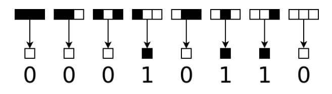
We can describe a 1D cellular automaton as a set of rewrite rules that act on a 1D array of bits over (discrete) time. To advance one generation, we iterate over memory and match the pattern around (below, \(n=3\)) each bit and replace it accordingly.
For some programs, predictable behavior emerges.
In theory, we could write a "simpler" program to output the same result; we can predict the state of any location in memory at a given time. In this sense, the pattern generated by the cellular automata is compressible.
However, some rules (famously, rule \(30\)) are "unpredictable" (although they may have some structure). There may be no way to predict the state of memory; executing the program is the only way to find out. So, the program cannot be "compressed" at all.
In general, there is no way to predict the behavior of a program from its description, even when that description is simple.
Rule \(30\) specifically is a universal computer; it can be used to execute any computation (proven in 2000), and is thus the simplest known Turing-complete system.
Mathematics is also, categorically, the study of consequences of simple sets of rules (axioms). Clearly, complex behavior can emerge from simple sets of axioms, so math may also be "incompressible", i.e. not amenable to general, overarching theories (sorry category theorists!).
Every program is a string (a finite length sequence of characters from a finite alphabet \(\Gamma\)). Strings are a really nice way to describe programs; before this, we used the naturals, which was just gross. Read the original proof of Gödel's incompleteness theorem if you don't believe me.
Since strings are finite, the set of all programs must also be finite. But since there are infinitely many strings, there are infinitely many programs.
This does NOT mean that every problem can be solved by a program though.
A decision problem is problem where it must be determined whether every string in an alphabet is "true" or "false" (e.g. graph isomorphism problem). Informally, a decision problem is a question that either has a true or false answer. This implies a subset, namely the subset of "true" strings. In fact, there is a one-to-one correspondence between subsets and decision problems.
decision : String -> boolIf we consider decision problems in general (i.e. over the set \(\mathcal{S}\) of all strings), we find that each subset of strings (i.e. each element of \(\mathcal{P}(\mathcal{S})\)) corresponds to exactly one decision problem. We know that \(\#\mathcal{S} < \# \mathcal{P}(\mathcal{S})\) even when \(\mathcal{S}\) is infinite, so there must be more decision problems than strings, and thus there must be more decision problems than programs.
We can't just compare the sizes of infinite sets "normally"; we find that sets have the same cardinality iff a bijection can be drawn between them.
Cantor's Theorem
TheoremThe set of decision problems is the power set of the set of strings, since each string can either be true or false. A decision problem is a subset of the set of all strings. Programs are also strings. Every decision problem being describable by a program implies a bijection from the set of strings to the power set of strings, which we've just shown can't exist. Thus, there are decision problems that aren't describable with programs.
Cantor's theorem and the result that some decision problems don't have a program to describe them are both non-obvious; both problems are proving non-existence in an infinite domain. It is not a coincidence that both proofs involved self-reference:
Allowing and utilizing self-reference often cuts to the core of questions, yielding both weird behavior and important results. Particularly, self-reference is a shortcut to finding contradictions.
As we've seen, it is possible to create universal programs (and relatedly, universal languages which can express any computation → whose interpreter must be a universal program). However, it is impossible to write a universal programming language in which every program halts. The existence of universal programs implies non-halting programs.
We use a diagonal proof. List all countably infinite programs expressible by the language \(p_1, \dots\), then through some traversal run each program with each program's string representation as input (a countably infinite traversal trivially exists). Define traversal \(V\) that acts as normal unless a program is run with itself as input, in which case it negates the result. \(V\) is a program we can write, so it is expressed by \(p_i\) for some \(i\in \mathbb{N}\), meaning we evaluate \(V(V)\) at some point. This calls \(V\) again, which eventually evaluates \(V(V)\), which calls \(V\) again, etc. Clearly, this program recurses forever and never returns.
Essentially, any language complicated enough to support universal computation also supports some recursive or loop structure, and thus infinite loops can be created in it.
Questions about the semantics (meaning/behavior) of programs are susceptible to halting-style diagonal arguments, and thus often provably impossible to answer in the general case, i.e. write a program to answer.
Undecidable Questions about Semantics
Examplegoto-branch loop exists; that type of non-halting behavior can be detected.These limits exist on every formal system, e.g. programming languages. Your static code analyzer can only get so good.
However, questions about syntax (description) are less susceptible to these arguments.
while loops are more powerful than those with just for loopsWait, why does this course have a real analysis co-req?
Before being able to use real numbers, we need to understand them, and thus we need to construct them. To bake an apple pie from scratch, one must invent the universe; we start by constructing \(\mathbb{N}\).
\(\mathbb{N}\) is constructed by the Peano axioms.
We extend \(\mathbb{N}\) to \(\mathbb{Z}\) by requiring closure under additive inverses.
We extend \(\mathbb{Z}\) to \(\mathbb{Q}\) by requiring closure under multiplicative inverses. \(\mathbb{Q}\) is defined as the classes defined by the equivalence relation \((a,b)\sim(c,d)\iff ad=bc\) over \(\mathbb{Z}\times \mathbb{Z}\), with definitions of addition, multiplication, etc. to match.
\(\mathbb{Q}\) is archimedean and dense in \(\mathbb{R}\), but almost all real numbers are not rational. Proving this is a nontrivial exercise in real analysis; we prove existence of an irrational number, namely \(\sqrt{2}\) as is customary.
Proof that \(\sqrt{2}\) is irrational
ProofAny equation involving addition, multiplication, and their inverses can be solved in \(\mathbb{Q}\), but equations of the form \(x^n=a\) aren't solvable in general. Adding radicals \(\surd\) to \(\mathbb{Q}\) doesn't solve everything either; polynomials of the degree \(5\) and higher aren't generally expressible in terms of the operations we have (a result of Galois theory). Again, we can define the algebraic numbers \(\mathbb{A}\) as the algebraic closure of the rationals, but not only does this not contain all of \(\mathbb{R}\) (i.e. transcendentals like \(\pi\) and \(e\)), but we now have members of \(\mathbb{A}\) not in \(\mathbb{R}\), e.g. \(\sqrt{-1}=:i\).
We finally construct \(\mathbb{R}\) from \(\mathbb{Q}\) by considering all the possible limits of (Cauchy) sequences of rational numbers, and including these in the number system as well. E.g. although \(e\) is transcendental, we do have \(e:=\displaystyle\lim_{n\to \infty}\left(1+\dfrac{1}{n}\right)^n\). \(\mathbb{R}\) is the closure of \(\mathbb{Q}\) under the inclusion of limits of cauchy sequences.
There's really no reason to stop here. We define the complex numbers \(\mathbb{C}\) as the algebraic closure of \(\mathbb{R}\), i.e. the set of solutions to any algebraic equations in \(\mathbb{R}\) (much like \(\mathbb{A}\) is a algebraic closure of \(\mathbb{Q}\)).
In general, new number systems are motivated by closure under some operation or construction. We can generalize the idea of a closure operator.
Not all numbers are computable, i.e. for which a terminating algorithm for approximating them to arbitrary precision exists. By definition, if a closed form limit exist, we can compute it. Clearly, it's ontologically difficult to describe an uncomputable number. But, since there are countably finitely many programs and uncountably infinitely many reals, most reals are uncomputable.
Clearly we can't use the cauchy sequences since we need infinitely many rationals to represent an uncomputable real, and dealing with limits is annoying for precise computation anyway. We have this problem with \(\mathbb{R}\) because its "closure operator" is real-analytic, as opposed to a clean, "algebraic" operator.
Cantor's Diagonal Argument
ProofAround this time, paradoxes were appearing in math that threatened the foundational assumptions of the time, namely that all of math could be built atop set theory:
The field of computer science emerged from a desire by the mathematical community to construct all of math from arithmetic on natural numbers, much like how \(\mathbb{Z}\), \(\mathbb{Q}\), \(\mathbb{R}\), etc. were constructed.
Church-Turing thesis
TheoremWe start by defining the primitives we will use to construct a theory of computation
A finite state computation is a computation that takes a string \(w\in \Sigma^{*}\) and either accepts or rejects it following computation by a finite automaton.
Intuitively, a finite automaton is defined by a set of states (what the computation has come to at this point in time) and a function that defines a new state based on the current state and the current input being read from the input string.
Finite Automaton (FA)
DefinitionAn FA can be expressed as a table indexed by the set of states and the set of characters that can form strings; the entries define the transition function at those coordinates.
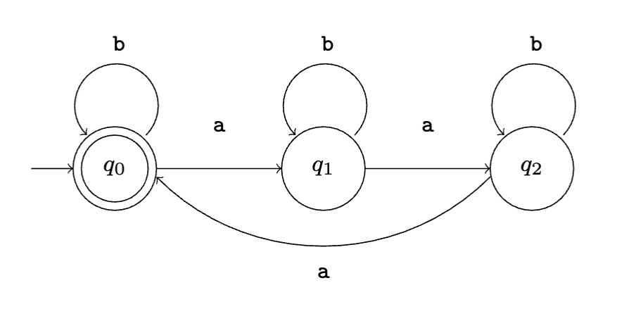
More commonly, an FA is expressed as a state diagram, where states are drawn as nodes and the transition functions is defined by arrows connecting the nodes. Accepting states are drawn with double stroke.
Computation
DefinitionSince we assumed the input string is of finite length and the execution is in lockstep with the input string's symbols, all computations will halt! In fact, if there are \(n\) input symbols, there will be exactly \(n-1\) steps in the computation; this property is very useful, e.g. in the proof of THM 2 later.
A state can be thought of as an equivalence class over the entire history of the computation. Namely, the representative of the "history class" is determined by its final state. In other words, there is no "memory" or "side effects" that affect how state is interpreted; behavior is determined entirely by the current state and input symbol
Given an alphabet \(\Sigma\), a language \(\Gamma\) is a subset of the set \(\Sigma^{*}\) of all strings, i.e. \(\Gamma\subseteq \Sigma^*\)
Examples of languages:
Constructing a FA to recognize a language will be familiar to anyone who has taken CMPUT 415.
A given automaton recognizes exactly one language, but a regular language has infinitely many FAs that recognize it (e.g. we can split edges, etc.)
The set of strings \(\Sigma^*\) of finite alphabet \(\Sigma\) is countably infinite, but since a program is characterized by which strings from \(\Sigma^{*}\) it accepts or rejects, the set of all languages over \(\Sigma\) is isomorphic to \(\mathcal{P}(\Sigma^{*})\), and thus is uncountably infinite. So, there are more languages than strings.
The set of all finite automata is also countably infinite since the input string, number of states and (therefore) size of transition functions are finite or countably infinite. By the same argument, there are more languages than finite automata. So, almost all languages are not regular.
Languages are isomorphic to decision problems over strings; languages \(\cong\) subsets of strings \(\cong\) decision problems \(\cong\) unary relations. In all of these cases, we can use the same \(|S| < |\mathcal{P}(S)|\) reasoning.
A regular operation is a binary operation \(\square : \mathcal{P}(\Sigma^{*}) \times \mathcal{P}(\Sigma^{*}) \to \mathcal{P}(\Sigma^{*})\) between languages that preserves regularity. I.e. if languages \(A\) and \(B\) are regular and \(\square\) is a regular operation, then \(A \, \square \, B\) is also a regular language.
| Operation Name | Symbol | Definition |
|---|---|---|
| Complement | \(\overline{\Gamma}\) | \(\overline{\Gamma} := \set{w \mid w \not\in \Gamma}\) |
| Intersection | \(\Gamma \cap \Lambda\) | \(\Gamma \cap \Lambda:=\set{w\mid w \in \Gamma \land w \in \Lambda}\) |
| Union | \(\Gamma \cup \Lambda\) | \(\Gamma \cup \Lambda:=\set{w\mid w \in \Gamma \lor w \in \Lambda}\) |
| Concatenation | \(\Gamma\Lambda\) or \(\Gamma \circ \Lambda\) | \(\Gamma \Lambda :=\set{ab\mid a\in \Gamma \land b\in \Lambda}\) |
| (Kleene) Star | \(\Gamma^{*}\) | \(\Gamma^{*}:=\displaystyle\bigcup_{n=0}^{\infty}\set{w_1 w_2 \dots w_n \mid w_i \in \Gamma}\) |
Theorem 1
TheoremTheorem 2
TheoremWe generalize finite state machines into non-determinism; we now differentiate between deterministic FAs (DFAs) and nondeterministic FAs (NFAs).
Nondeterministic Finite Automaton (NFA)
DefinitionWe define \(\varepsilon\) as the null character, which allows \(\varepsilon\)-transitions (spontaneous state transitions) that don't process the next input symbol. We define \(\Sigma_\varepsilon := \Sigma\cup \set{\varepsilon}\).
Generalizing \(\delta\) from a function to a relation is what makes an automaton non-deterministic; a function is a special kind of relations where each "input" uniquely determines an output (i.e. all the subsets contain a single element), whereas a relation allows multiple elements that may be freely chosen between for a given "input".
Since a given state/input pair may have multiple successors, the shape of our program's execution generalizes from an execution sequence to an execution tree of state/input pairs, which is defined analogously to an execution sequence. Program \(M\) accepts string \(w\) iff the execution tree contains a configuration with an accepting state.
Two machines \(M_1\) and \(M_2\) are equivalent if they recognize the same language.
DFAs and NFAs are Equivalent
TheoremBy corollary, the following statements are logically equivalent:
By establishing an equivalence between DFAs and NFAs, we can use the new primitives of DFAs to prove statements NFAs/regular languages. In particular, we use \(\varepsilon\)-transitions to show that regular languages are closed under union, concatenation, and the Kleene star.
Theorem 3
Theorem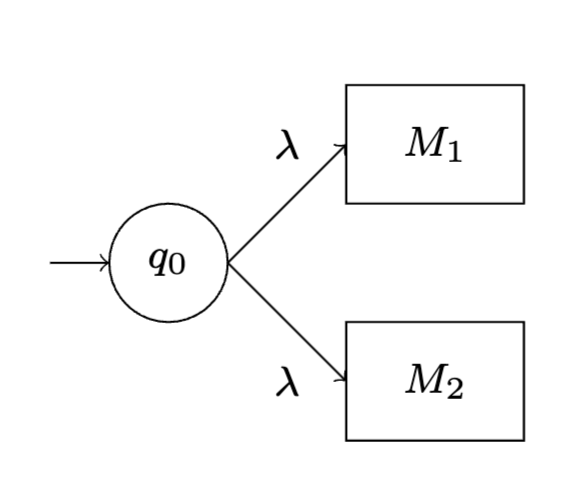
Theorem 4
Theorem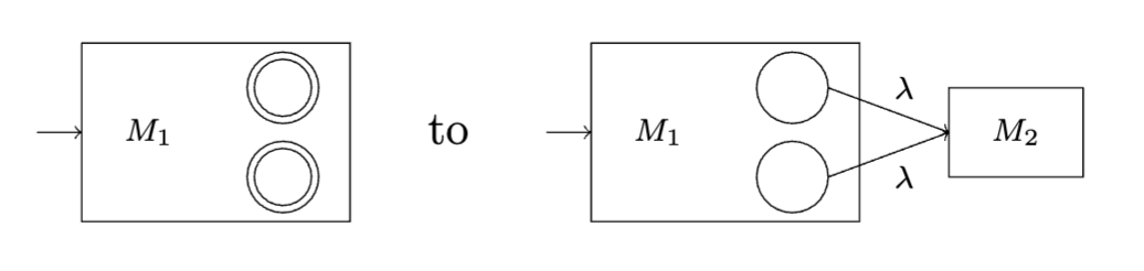
Theorem 5
Theorem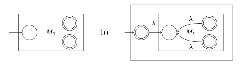
A regular expression is an expression formed of regular operators operating on regular languages. Thus, the language of regular expressions is itself a regular language; we see regular expressions as a meta-language that can construct regular languages syntactically, as opposed to the "semantic" way (listing the strings in the language).
We recursively (in order of precedence) define \(R\) as a regular expression if
We define \(\mathcal{L}(R)\) as the language specified by regular expression \(R\), implicitly with alphabet \(\Sigma\). We also define the shorthand \(R=\Sigma\) for shorthand \(R=\sigma_1 \cup\dots\cup \sigma_{|\Sigma|}\), i.e. the language formed by the symbols of \(\Sigma\).
Examples of regular expressions (for \(\Sigma=\set{0,1}\))
Identities for Regular Expressions
LemmaRegular Expressions and Regular Languages are Equivalent
TheoremProof sketch \(\impliedby\): We simply construct and compose NFAs as we did when we defined the regular operators; we have more or less proven everything we need already. For the base cases, we have:
We must define more concepts to prove \(\implies\).
Generalized NFA
DefinitionA GNFA accepts input \(w\) iff there exists a sequence \(q_0, c_1,\dots,c_{k-1},q_a\) of configurations where \({w_{i+1}\in \mathcal{L}(\delta(c_i, c_{i+1}))}\) for \(i\in\set{0, \dots, k-1}\). So, moving to a new state requires that the regular expression defined by the pair of states (in \(\delta\)) recognizes the input that it consumes.
DFAs are a subset of GNFAs
LemmaReduction Procedure for a DNFA
AlgorithmOtherwise, choose a state (that isn't the initial or final one) and contract (in the graph theory sense) the DNFA with respect to that state. This requires coalescing the regular expression (where \(q_\times\) is the state to be remove and \(q_i,q_j\) any pair of REs on "either side" of \(q_\times\)):
We keep contracting until there are only two states left.
\(\mathcal{L}\) is Invariant under Reduction
Lemmadiagrams
TODO: add a table with all the NFA diagrams to the appendix in a "constructing NFAs from regular expressions section
The language \(\Gamma_1:=\set{0^{n}1^{n}\mid n\geq 0}\) (i.e. language formed by a substring of \(0\)s followed by a substring of \(1\)s of the same length) is cannot be regular because as \(n\to \infty\), we would need an infinite amount of states (or memory) to "remember" \(n\).
Clearly, any finite language is regular because we can "hard-code" each string into the FA directly, so all non-regular languages must be infinite. Furthermore, if a language is infinite, it has no bound on the length of strings, so its regular expression representation must use a Kleene star. Specifically:
Pumping Lemma for Regular Languages
TheoremI.e. for sufficiently long strings in \(\Gamma\), there is always a substring that can be repeated arbitrarily.
Proof sketch (general idea): Let \(\Gamma\) be regular and recognized by DFA \(M\). Pick \(p = |Q_M|\). If we have some string \(w\) that is longer than \(p\), the computation of \(M\) with \(w\) as input must pass through at least one state (denoted \(q_!\)) twice by the pigeonhole principle, and thus a loop exists. Let \(\sigma_!\) be the input symbol when the loop is first encountered. If we were traversing the DFA "for fun", we could choose to follow the loop as many times as we wanted. Thus, any modification of \(m\) from arbitrarily duplicating the substring corresponding to the loop will also be recognized by \(M\).
Note that the pumping lemma is necessary for regularity, but not sufficient: there are irregular languages that conform to the pumping lemma.
If a language is regular, it must adhere to the pumping lemma. Thus, by contrapositive, if a language \(\Gamma\) has a string \(w\) such that all \(w=xyz\) decompositions have some \(i\) such that \(xy^{i}z\not\in \Gamma\), then \(\Gamma\) can't be a regular language.
Example: Consider \(\Gamma_1:=\set{0^{n}1^{n}\mid n\geq 0}\); assume towards contradiction that it is regular. Then a DFA \(M_{\Gamma_1}\) with some \(p\in \mathbb{N}\) states that recognizes \(\Gamma_1\) exists. Consider the string \(w_\times:=0^{p}1^{p}\in \Gamma_1\). Any decomposition \(w_\times = xyz\) where \(|y|>0\) and \(|xy|\leq p\) implies \(y=0^{k}\) for some \(k\leq p\), since \(xy\) itself must be a string of \(0\)s (since there are \(p\) \(0\)s). But, since all the \(1\)s in the string are in \(z\), the string \(xy^{2p}z\) must have more \(0\)s than \(1\)s, and thus \(xy^{2p}z\not\in \Gamma_1\). If \(\Gamma_1\) were regular, we would have \(xy^{2p}z\in \Gamma_1\) by the pumping lemma. So, \(\Gamma_1\) is not regular.
Closure!
If \(\Box\) is a regular operator and \(\Gamma_{\text{Reg}}, \Lambda_{\text{Reg}}\) are regular languages, then we know \(\Xi:=\Gamma_{\text{Reg}} \Box \Lambda_{\text{Reg}}\) is also regular. Thus, by contrapositive, if \(\Xi_{\lnot \text{Reg}}:=\Gamma\Box\Lambda\) is not a regular language, then at least one of \(\Gamma\) and \(\Lambda\) isn't a regular language as well. More specifically, id \(\Xi_{\lnot \text{Reg}}:=\Gamma_\text{Reg}\Box\Lambda\) for regular \(\Delta_\text{Reg}\), then \(\Lambda\) must not be regular.
So, to prove some \(\Gamma\) is not regular, we define a language known not to be regular as the product of a regular operation on a regular language and \(\Gamma\).
Example: Consider \(\Gamma_2\) as the language of strings with alphabet \(\Sigma=\set{0,1}\) that have the same number of \(0\)s as \(1\)s. Note that \(\Gamma_1=\Gamma_2 \cap L(0^{*} 1^{*})\). Clearly \(L(0^{*} 1^{*})\) is regular (it is defined by a regular expression), and we know that \(\Gamma_1\) is not regular. So, \(\Gamma_2\) must be irregular as well.
Example: Consider \(\mathsf{R}\) as the language of regular expressions (specifically, where \(\varepsilon\) is a valid regular expression) and \(\mathsf{P}\) as the language consisting of strings of parens, i.e. \(\mathsf{P}:=\set{(,)}^{*}\). Clearly \(\mathsf{P}\) is regular. We note that \(\mathsf{R}\cap\mathsf{P}\) is the set of balanced parenthesizations; it is common knowledge that this language is not regular. Thus, since \(\mathsf{R}\cap\mathsf{P}\) is not regular but \(\mathsf{P}\) is, it must be that \(\mathsf{R}\) is not regular.
Note: closure arguments are recursive; proving a language is regular is achieved by proving some other (presumably simpler) language is regular. Using the pumping lemma is the only "base case" that we have other than direct proof, so all roads will lead to it eventually.
Finite-state computation can be generalized into a more powerful model of computation by removing the requirement that the set of states is finite. Of course, the program specification must still be finite, so we can't just use an infinite lookup table. But, if the state transition function/relation has structure, it may have a finite amount of information, and thus could be expressed finitely.
We extend our model by adding finitely-addressable memory (i.e. countably infinite memory, where addresses are in \(\mathbb{N}\)) that can be used to store the state of the computation.
A natural data structure to store in memory is a stack, where a stack counter stores the address of the top of the stack. Thus, although the stack can grow without bound, changes are local, i.e. always occur at the stack pointer, which moves "continuously in \(\mathbb{N}\)".
At each step of the computation, a pushdown automaton will advance \(1\) step on the input string, read the character, pop from the stack, and use this information to advance to a new state and push another symbol onto the stack.
Deterministic Pushdown Automata (DPDA)
DefinitionI.e. it is an extension of a DFA to include a stack, which has its own alphabet and factors is a dimension of the transition function.
More on the transition function \(\delta\):
As with before, a configuration is a triple \(c=(q \in Q, u\in \Sigma^{*}, s\in \Gamma^{*})\) and an execution trace of string \(w\in \Sigma^{*}\) is the (unique) sequence of configurations generated by the computation on \(w\). \(M\) accepts \(w\) if it reaches a configuration \(c_\ell=(q_k , w, s)\) where \(q_k\in F\).
Clearly, the set of FAs is isomorphic to the subset of DPDAs that simply don't interact with the stack, i.e. given by \(M_\text{FA}:=(Q, \Sigma, \varnothing, \delta, q_0, F)\).
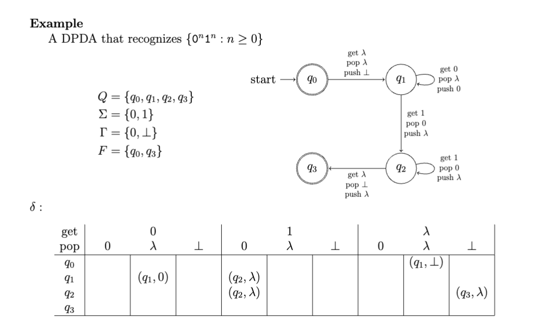
Fundamentally, stacks let us traverse trees; in the degenerate cases of a tree being a path (i.e. a linked list, for the data structures brainrot enjoyers among us), a stack lets us count whatever patterns we want. So, languages like \(\set{0^{n}1^{n}\mid n\geq 0}\) can be recognized by DPDAs:
Deterministic Pushdown Automata (PDA)
DefinitionLike before for DFA → NFA, \(\delta\) is extended such that a given configuration could lead to multiple other configurations, or none at all. So, computations are not deterministic and the execution structure is a tree, not a sequence.
Also like before, since the the set of functions \(A \to B\) is a subset of of the set of relations over \(A\times B\), the set of DPDAs is a subset of the set of PDAs.
However, unlike before, PDAs are strictly more powerful than DPDAs; they are not equivalent like DFAs and NFAs are! So, adding a stack augments the power of NFAs more than the power of DFAs.
I'm guessing some of this will get covered later remove if it is
With the memory model, we can use a lot more than just one stack:
Relevant XKCD: https://xkcd.com/1090/
Reese lecture :))
So far, we've used specifications to generate target languages and defined programs that can mechanically recognize strings against a specification. For a given "language class", bijective pairs of specification and program structures exist, i.e. where every specification can be implemented as a program and every program implements a specification.
This pattern will continue: context-free languages are described by context-free grammars and can be recognized by pushdown automata (more on this in this lecture)
Context-Free Grammar
DefinitionA derivation in a CFG \(G\) is performed by picking a start variable and iteratively substituting variable occurrences using production rules. Each derivation implies a parse tree whose nodes are strings (possibly containing variables) and whose edges are production rules.
A string \(w\) is generated by \(G\) (denoted \(S_G \overset{*}{\Rightarrow} w\)) if it can be derived from \(G\) and only contains terminals. The language \(\Gamma_G\) of grammar \(G\) is set set of strings generated by \(G\), i.e. \(\set{w\in \Sigma \mid S \overset{*}{\Rightarrow} w}\); if \(G\) is a context-free grammar, then \(\Gamma_G\) is a context-free language. A context-sensitive language is a language that isn't context-free.
Context-free grammars generalize regular expressions; CFGs are to pushdown automata as regular expressions are to finite automata. The extra power of CFGs comes from self-reference; we are allowed to bind a name to a syntactic construction (rule) and reference it later, which opens the door to recursion and the computational oomph that it entails.
Our regular (lol) question persists: given a language, can we write a regular expression grammar for it?
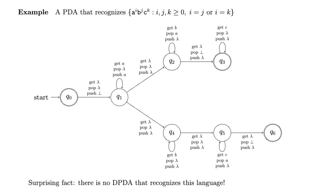
Canonical examples of context-free grammars that aren't regular include the language of palindromes (over some alphabet \(\Sigma\)), the language of well-balanced parenthesizations (the Dyck language), and languages like \(\set{a^{n}b^{n}\mid n\in \mathbb{N}}\).
Grammars are also notable because they can be used to describe programming languages (take CMPUT 415 for more on this in practice). Most languages are mostly context-free, although many have context-sensitive quirks.
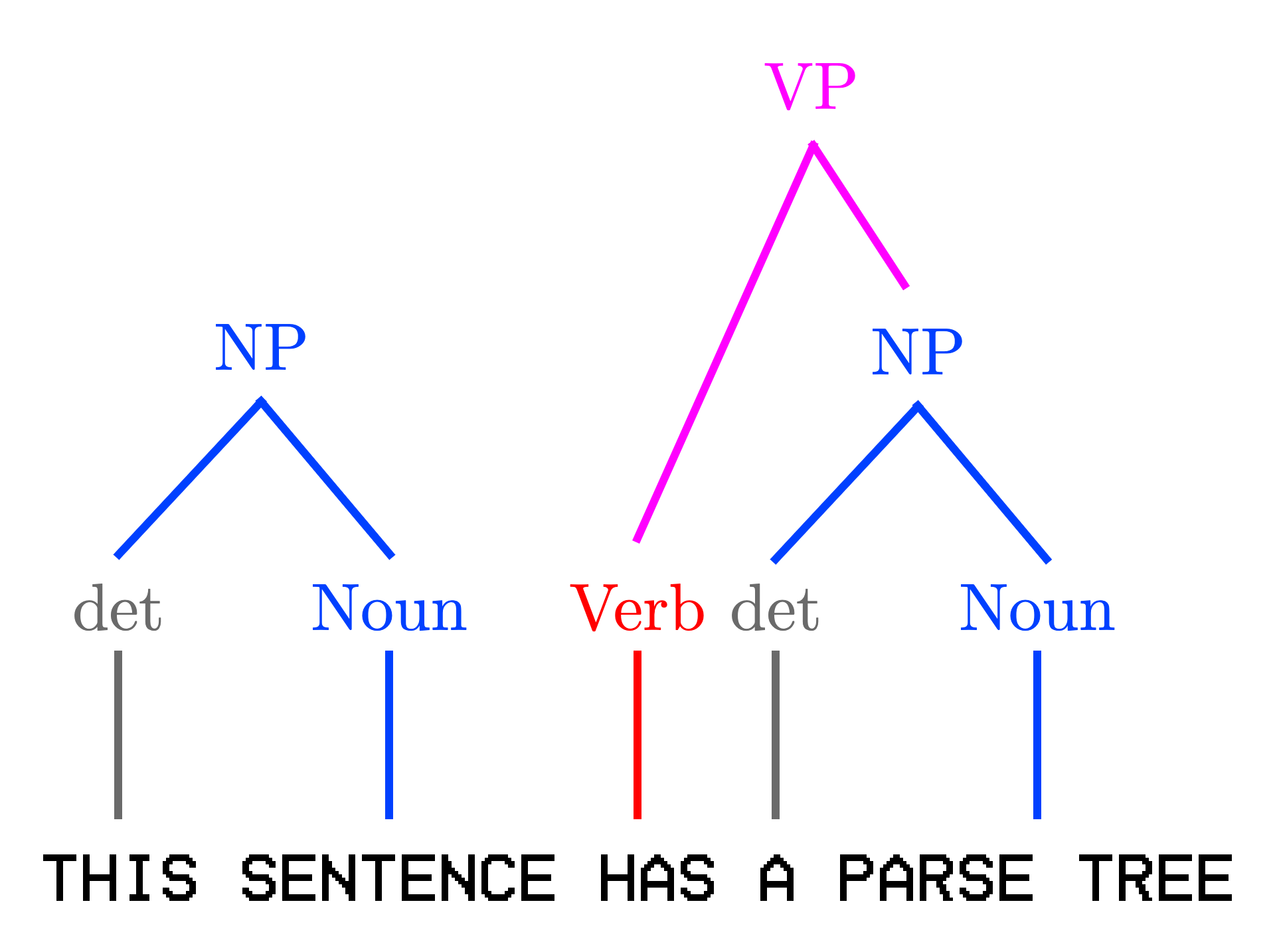
CFGs also let us create decent models of natural language:
For larger grammars, it makes sense to write them over multiple lines, and adopt "code" typesetting (as opposed to mathematical typesetting). Backus-Naur form is standard, but I prefer to use ANTLR's syntax for its brevity and applicability. Note that ANTLR4 has some syntactic sugar, like regular expressions as nonterminals.
ALL_CAPS and rules are lowercaseExample: Grammar for common LISP
Adapted from https://github.com/antlr/grammars-v4/blob/master/lisp/lisp.g4
lisp_ : s_expression+ EOF;
s_expression
: ATOMIC_SYMBOL
| '(' s_expression '.' s_expression ')'
| list
;
list : '(' s_expression+ ')';
ATOMIC_SYMBOL: LETTER ATOM_PART?;
ATOM_PART : (LETTER | NUMBER) ATOM_PART;
LETTER: [a-z];
NUMBER: [1-9];
WS: [ \r\n\t]+ -> skip;If we must use math notation, we can coalesce rules starting with the same variable by writing them as alternatives, delimited by \(\mid\). So, \(\set{S \to \varepsilon, S \to (S), S\to SS}\) can be written succinctly as \(S\to \varepsilon\mid (S) \mid SS\).
CFGs are a superset of regular expressions
TheoremBy corollary, the class of regular languages is a subset of the class of context-free languages.
Closures of CFGs
TheoremProof: for each operator \(\square\), we consider the language formed by combining the sets of variables and rules of the two languages \(\Gamma\) and \(\Lambda\); we define \(\Gamma\, \square \, \Lambda\) to have start variable \(s\).
Each time, just like with regular expressions, we defer the operations to the corresponding constructs for building grammars.
Whoopsie, made a oopsie
WarningA grammar \(G\) is ambiguous if the same terminal string can be derived in different ways, i.e. if a given string in the language \(\Gamma_G\) has multiple different parse trees.
Context-free languages can be ambiguous; a context-free language is inherently ambiguous if every grammar that describes it is ambiguous.
Canonical form time 😎
A context-free grammar is in Chomsky normal form when every rule is of the form \(A \to BC\), \(A \to a\), or \(S \to \varepsilon\) for variables \(A,B,C\) (where \(B,C \ne S\)) and terminal \(a\).
Chomsky normal form is a normal form
TheoremWe prove by construction; the following is a complete list of language-preserving transformations over grammatical rules:
We can convert a grammar to Chomsky normal form by repeatedly applying these rules until no replacements can be made; the number of such replacements is finite. So, we are performing fixpoint iteration.
Chomsky normal form is useful because it requires parse trees to be binary. Thus, there is a strong relation between the length of a string and the height and/or number of nodes in its parse tree.
Our central theorem:
PDAs and CFGs are Equivalent
TheoremFor this proof, we use the notion of a generalized pushdown automaton (GPDA), which can push entire strings to the stack instead of just characters.
Equivalence of GPDAs and PDAs
AlgorithmWe also define the restricted pushdown automaton (RPDA), which is a PDA with a single accepting state, empty stack upon termination, and where every stack action is either a single push or single pop.
Equivalence of RPDAs and PDAs
TheoremWe can draw an equivalence between the steps in a leftmost derivation performed in \(G\) and a sequence of configurations in some PDA \(M\). Then, we push build a string by pushing and popping strings on \(M\)'s stack.
We define a GPDA that traverses through a string and pushes the corresponding rule bodies from variables to the stack. In this way, it performs the leftmost derivation. So, an accepting sequence of configurations exists in \(M\)'s computation of \(w\) if and only if a leftmost derivation of \(w\) exists in \(G\).
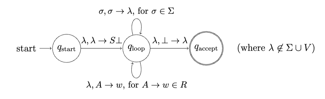
We know that GPDAs are equivalent to PDAs, so can construct a PDA with the same behavior as the above GPDA. So, we've shown that given a CFG, we can construct a PDA that recognizes a string if and only if it can be generated by the CFG.
We prove again by construction. Given an RPDA, we can construct a CFG as follows:
review this and add more intuitive explanation!!
First, we claim that if \((q_a, w, \varepsilon) \overset{*}{\to} (q_b, wx, \varepsilon)\), in the RPDA/PDA, then \(A_{q_a,q_b}\overset{*}{\Rightarrow} x\) in the CFG, then the converse. Both can be proven by induction; our base case is when both configurations are actually the same (i.e. where \(x=\varepsilon\)).
add proofs!!
Although they are more powerful than FAs, PDAs are not universal computers either; there exist algorithms that can't be adapted for PDAs. Since PDAs are equivalent to CFGs, we will reason about CFGs below.

Pumping Lemma for CFGs
TheoremI.e. for sufficiently long strings in \(\Gamma\), there is always a substring that can be repeated arbitrarily.
Since \(G\) has a finite number of variables and each substitution increases the size of a generated string by a finite amount, there is an upper bound (here, \(p\)) on how long a string can get when each rule substitutes a given variable at most once. Thus, if a string is longer than this \(p\), there must be variable \(A\in V\) that gets substituted more than once over the course of a derivation, i.e. a rule \(R\ni \mathcal{R} : A \to \dots\) is applied more than once.
We consider the possible height of a parse tree for a string in language \(\Gamma(G)\) for CFG \(G\).
In this context, the branching factor \(b\) of the parse tree is the maximum length of an RHS rule in \(G\); a tree of height \(h\) can have at most \(b^{h}\) leaves. Also note that a string of length \(\ell\) needs ==height at least \(b/\ell\), and thus height of at least \(\log_b{\ell}\) to generate.==
If a rule isn't repeated, a tree of height at most \(|V|\) can exist. So, if \(h \geq \log_b{\ell} \geq |V| + 1\) \(\iff b^{h}\geq \ell \geq b^{|V| + 1}\), then some path \(S \to \text{leaf}\) exists where some variable \(A\) repeats.
Pick \(p:=b^{|V| + 1}\) and string \(w\in \Gamma(G)\) of length \(\ell\) where \(\ell \geq p \implies \ell \geq b^{|V|+1} \geq b^{|V|}+1\). The smallest (by number of nodes) parse tree for \(w\) must have height at least \(|V|+1\), and thus some path \(T\) of length \(\geq |V|+1\). So, by pigeonhole principle, some variable \(A\) exists that repeats in the path; denote the instances \(A^1\) and \(A^2\).
We can partition \(w\) into \(uvxyz\) where \(A^{1}\) produces \(vxy\) and \(A^{2}\) produces \(x\).
The strategy for proving a language isn't context-free is more or less the same as proving it isn't regular using the pumping lemma: we
E.g. it can ergonomically be proven that \(\Gamma:=\set{ww \mid w\in \set{0,1}^* }\) is not context free by choosing string \(w:=0^{p}1^{p}0^{p}1^{p}\) (where \(p:=p_G\)).
Proving via closure under operations, while strictly possible, isn't as useful for context-free languages as it is for regular languages because context-free languages aren't closed under intersection. The most useful closure arguments involve intersections of regular languages.
q_cross and q_checkmark for accept/reject, better underline syntax, pick suitable font for left/right
Earlier, we generalized from FAs to PDAs by equipping them with a stack. Now, we can further generalize PDAs to a Turing machine by replacing the stack with a more general data structure, i.e. one that can simulate a stack. Specifically, TMs have a tape: an infinite, finitely addressable tract of memory cells that an automaton can read from, write to, and move along in either direction.
Just like for PDAs, although their memory is unbounded, Turing machines allow infinite decision problems to be defined finitely. In fact, Turing machine are the strongest such automata:
Church-Turing Thesis (Lite)
TheoremCoding an algorithm as a Turing machine is the theoretical CS equivalent of writing a computer program in assembly (or by pushing transistors around). In both cases, you are reaching into the entrails of a machine and building your program bit by bit by bit. Designing Turing machines is hard for the same reason that writing assembly is hard.
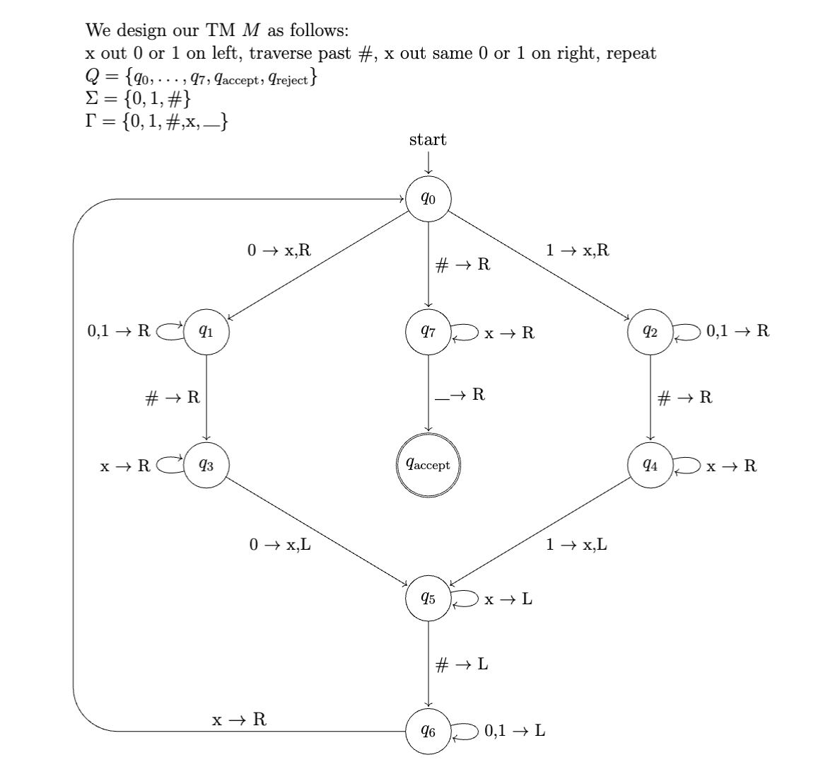
We also notice a pattern while designing Turing machines: most programs consists of a search/seek operation, then a write operation, then search/seek, then write, etc.
Turing Machine (TM)
DefinitionThe state of a TM at a moment in time (a configuration) can be described as \(aqb\) where \(a,b\in \Gamma^{*}\) are the strings that list the characters on either side of the read/write head and \(q\in Q\) is the current state. A computation is a "physically valid" sequence of configurations.
Turing machine \(M\) accepts string \(w\) if \(M\) can reach configuration \(c_k=uq_\text{accept}v\), for \(k\in \mathbb{N}\) (i.e. \(k < \infty\)) and strings \(u,v\in \Gamma^{*}\). \(M\) rejects if it can reach a configuration \(c_k=uq_\text{reject}v\). If neither of these happen, the computation does not halt on \(w\).
Again, for Turing machine \(M\), we define \(\mathcal{L}(M)\) as the language of string accepted by \(M\). So, \(\overline{\mathcal{L}(M)}\) is the language of strings that are either rejected by \(M\) or for which \(M\) doesn't halt.
Turing machine \(M\) decides \(\mathcal{L}(M)\) iff \(M\) halts for all possible input, i.e. for all \(w\in \Sigma^{*}\).
Language \(\Lambda\) is Turing-recognizable if \(\Lambda=\mathcal{L}(M)\) for some Turing machine \(M\). \(\Lambda\) is Turing-decidable if it is recognizes by a Turing machine \(M\) that halts on every \(w\in \Sigma^{*}\supseteq \Lambda\).
As with every model of computation we've seen so far, non-determinism is achieved by generalizing the transition structure \(\delta\) from a function to a relation. Indeed, a non-deterministic Turing machine is defined the same way:
Non-deterministic Turing Machine
DefinitionAgain, like before, computations for nondeterministic Turing machines take the form of trees.
lots of this wording kinda sucks/isn't concise
The "basic" Turing machine described earlier can simulate any extended Turing machine below. So, when we reason about basic Turing machines, we can augment them with any of these extensions without weakening our statement:
Moreover, we can further restrict the basic model without giving up computational power
Every time we see a stay action, we simulate it with a left \(\mathsf{L}\) movement, then a right \(\mathsf{R}\) movement. The initial left movement writes the new symbol to the initial space; the right movement doesn't draw a new symbol.
At any given point, we have passed some finite number \(n\) of configurations; our input string \(w\) has some finite length \(|w|=m\) as well. So, at every point in a computation, there is some \(M \leq w + m\) such that every symbol past address \(M\) on the tape is a blank.
To insert, we loop from our current position. Each iteration, we keep track of the current symbol and overwrite it with the previous one, moving back then forward to keep track of the symbols. Eventually, we reach \(M\); we loop back to our original position without changing everything.
To delete, we follow a similar process, but we replace the current symbol with the following one. This also requires taking two steps forward and one step back each iteration.
There are a few ways we could go about this.
Idea \(1\): we define some delimiter symbol \(\#\) to separate the different tape models on our single tape. We also define a symbol \(\nabla\) that denotes the current position of our simulated read/write head. Each time we want to make a change to a tape, we
Idea \(2\): Define tape \(1\) as the cells of the tape equal to \(1\) \(\mod k\), tape \(2\) as the cells equal to \(2\) \(\mod k\), etc. Then, for a given tape, travel to the correct offset and navigate left and right by moving \(k\) spaces.
Strictly speaking, idea \(1\) is stronger because it can simulate an unbounded/arbitrary/changing number of tapes, whereas idea \(2\) can only support a fixed \(k\).
As we have seen, non-deterministic Turing machines have configuration trees. Briefly put, we can traverse this configuration tree with breadth-first search. Although this tree may have infinite depth, it has finite width (is this the term?), so BFS will reach every possible configuration eventually.
We can simulate a non-deterministic Turing machine \(\tilde{M}\) with \(3\) tapes:
Each loop, we increment the location in the tree according to BFS. Then, we simulate \(\tilde{M}\) from the point where we are currently located. If our simulation accepts, we return \(\text{accept}\); if our simulation rejects, we move on to the next location in the tree.
We've seen that a basic Turing machine can simulate any program with access to infinite, finitely addressable external storage, which is a reasonable abstraction for familiar kinds of computing systems. We've also seen that a basic Turing machine can simulate any algorithm, i.e. any mechanical procedure.
Now, we want to know:
This will help us understand the corresponding limits of Turing machines via the equivalence established by the Church-Turing thesis.
Describing Turing machines is the theoretical CS equivalent of writing machine code from scratch; it is the lowest possible level to describe a procedure. But, just like programmers (generally) choose not to express their ideas in assembly, we may opt to use higher-level descriptions of algorithms instead, as allowed by the Church-Turing thesis.
We assume that all inputs are strings and that any sort of object we might wish to use as input (e.g. a number, another program, etc) can be described as a string. Given object \(O\), the string description of \(O\) is denoted \(\langle O \rangle\).
As we've seen each new family of models of computation (first finite automata, then pushdown automata, then Turing machines), we've noticed that each new model can simulate the previous one. This leads concentric sets of corresponding languages; a widely-accepted (sub)-taxonomy is known as the Chomsky Hierarchy.
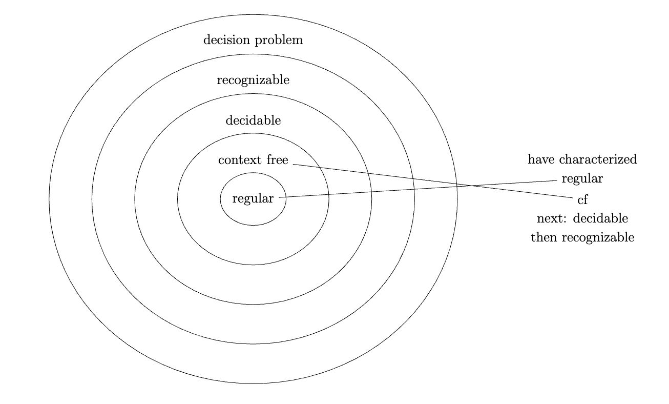
better disambiguation about chomsky hierarchy
Recall: a problem is decidable iff a halting algorithm exists that will accept or reject it.
Earlier, we constructed languages as a structure to collect and reason about sets of strings (sometimes with respect to a global alphabet \(\Sigma^{*}\)). A striking feature of theoretical CS is how the same structural patterns are repurposed over and over: equivalence, abstraction, reduction. So, reasoning about language classes and meta language classes are natural progressions.
A language class (or model of computation) \(\mathcal{M}\) is a set of languages. Language classes are an effective way to refer to sets of all possible types of structures.
A meta language class (with respect to \(\mathcal{M}\)) is a language classes of descriptions of languages that have some property with respect to \(\mathcal{M}\).
| Symbol | Name | Set construction |
|---|---|---|
| \(\text{A}_\mathcal{M}\) | Acceptance problem for \(\mathcal{M}\) | \(\set{\langle {M},w \rangle\mid M\in \mathcal{M} \text{ accepts or generates }w}\) |
| \(\text{E}_\mathcal{M}\) | Emptiness testing problem for \(\mathcal{M}\) | \(\set{\langle {M}\rangle\mid M\in \mathcal{M} \text{ has } L(M) = \varnothing}\) |
| \(\text{EQ}_\mathcal{M}\) | Equivalence testing problem for \(\mathcal{M}\) | \(\set{\langle {A},B \rangle\mid A,B\in \mathcal{M} \text{ such that } L(A)=L(B)}\) |
| \(\text{ALL}_\mathcal{M}\) | All string testing problem for \(\mathcal{M}\) | \(\set{\langle {M}\rangle\mid M\in \mathcal{M} \text{ has } L(M) = \Sigma^*}\) |
We cover decidability results for languages classes pertaining to structures we've already seen. Below, we assume \(M\) is an arbitrary "member" of the language class. We also assume that we've checked if \(M\) is well-formed; trivially, we can use a TM to check this before the principal computation
\(\text{A}_\text{DFA}\) is decidable
TheoremSince DFAs must halt (i.e. when they have consumed all their input), we can simply use a TM to simulate \(M\) on \(w\) given a description \(\langle M,w \rangle\). If this simulation ends on an accept state, the TM accepts. Otherwise, it rejects.
We simulate by building a model of \(M\) from \(\langle M \rangle\) in our TM, then keeping track of \(M\)'s current state and the current input position in \(w\).
\(\text{A}_\text{NFA}\) is decidable
TheoremWe construct a TM that converts the NFA to a DFA (\(O(2^{n})\)), then inherit from the fact that \(\text{A}_\text{DFA}\) is decidable.
\(\text{A}_\text{RE}\) is decidable
TheoremAgain, we construct a TM that converts the regular expression to an equivalent DFA, then inherit from the fact that \(\text{A}_\text{DFA}\) is decidable.
\(\text{E}_\text{DFA}\) is decidable
TheoremEssentially, we want to search all the possible paths from the initial state \(q_0\) and see if any end on accepting states. This is done by marking \(q_0\), then iteratively marking every state that can be reached from \(q_0\) by consuming input until a fixpoint is reached. If (at some point) we reach an accepting state, we reject. Otherwise, if we reach a fixpoint without accepting states, we accept.
\(\text{EQ}_\text{DFA}\) is decidable
TheoremGiven \(\langle A,B \rangle\), we construct new DFA \(C\) that decides \(L(A)\,\triangle\, L(B)\), where \(\triangle\) is the symmetric difference operator (set-theoretic XOR) defined by \(S \,\triangle\, T := (S\cup T) \setminus (S\cap T)\); such a \(C\) must exist because regular languages are closed under union, intersection, and complement. Then, since \(\text{E}_\text{DFA}\) is decidable, we decide whether \(L(C)=\varnothing\). Since \(L(C)=\varnothing\iff L(A)=L(B)\) by construction, we have decided either \(L(A)=L(B)\).
Bound on derivation size for a CFGs in CNF
Lemma\(\text{A}_\text{CFG}\) is decidable
TheoremNote that we can't just try every derivation, since there could be infinitely many. If that were the case, our procedure wouldn't halt for \(w\not\in L(G)\).
Instead, we derive \(G\) from description \(\langle G \rangle\), then convert it into its Chomsky normal form (denote with \(\tilde{G}\)). From the bound introduced above, we know our derivation has exactly \(2n-1\) steps, so we essentially search a tree of bounded width (since the CFG is finite) of (bounded) height \(2n-1\). If we find a path that generates our input string, we accept; otherwise, we reject.
\(\text{A}_\text{PDA}\) is decidable
TheoremAgain, we can't just simulate the PDA directly, since PDAs don't always terminate. Instead, we construct the PDA's corresponding CFG, then inherit from the fact that \(\text{A}_\text{CFG}\) is decidable.
\(\text{E}_\text{CFG}\) is decidable
TheoremAgain, we can't just search through strings, since we wouldn't halt if the language is indeed empty.
Instead, we proceed similarly to how we determined \(\text{E}_\text{DFA}\). We mark all of the terminals, then iteratively mark any rules whose bodies consists entirely of marked atoms, repeating until we reach a fixpoint. If the initial rule \(S\) has been marked, we reject; otherwise, we accept.
Note: We can't use our union/intersection/complement proof strategy to determine if \(\text{EQ}_\text{CFG}\) is decidable, since context-free languages aren't generally closed under intersection and complement. In fact, \(\text{EQ}_\text{CFG}\) is unrecognizable.
So far, we've proven that meta language classes are decidable. We will see examples and proofs of languages that aren't decidable.
\(\text{A}_\text{TM}\) is not decidable (i.e. is undecidable)
TheoremProof: assume towards a contradiction that \(\text{A}_\text{TM}\) is decidable. Then, there exists TM \(D\) that decides whether \(\langle M,w \rangle\in \text{A}_\text{TM}\). Define TM \(\text{Evil} : \langle M \rangle\mapsto \lnot D(\langle M, \langle M \rangle \rangle)\), which returns the opposite of output of \(D\) when run with some \(\langle M, \langle M \rangle \rangle\) as input. Consider \(\text{Evil}(\langle \text{Evil} \rangle)\), which reduces to \(\lnot D(\langle \text{Evil}, \langle \text{Evil} \rangle \rangle)\).
Thus, by contradiction, no such \(D\) can exist. Thus, \(\text{A}_\text{TM}\) is undecidable.
We can view this proof as a diagonalization argument. We enumerate all (countably many) machine descriptions \(\langle M_1 \rangle, \langle M_2 \rangle, \dots, \langle\text{Evil} \rangle, \dots\) as the inputs (columns), and machines \(M_1, M_2, \dots, \text{Evil}, \dots\) as the columns. As we will in the columns, we see the row corresponding to \(\text{Evil}\) has entries \(\lnot D_{k,1}, \lnot D_{k,2}, \dots\). We will be unable to fill in the entry for \([\langle \text{Evil} \rangle, \text{Evil}]\).
\(\text{A}_\text{TM}\) is recognizable
TheoremI.e. it is possible to construct a universal Turing machine.
Proof: trivially, given the description \(\langle M \rangle\), we construct a TM that simulates \(M\) on input \(w\). If this simulation hits an accept state we accept, and if it hits a reject state, we reject. By the definition of "recognizability", we don't need to worry about the case where the simulation of \(M\) doesn't terminate.
We say Turing machines are universal.
A language \(L\) is co-recognizable if its complement \(\overline{L}\) is recognizable.
Decidable iff recognizable and co-recognizable
TheoremAs a corollary:
\(\overline{\text{A}_\text{TM}}\) is not recognizable (i.e. not recognizable)
TheoremIf language \(\Lambda\) is known to be undecidable, and a decider for language \(\Gamma\) can be adapted to decide \(\Lambda\), then we can conclude (by contradiction) that \(\Gamma\) must also be undecidable. This is a proof by reduction.
We often reduce to the Halting problem since it is the canonical undecidable problem.
We define the halting problem over a meta-language of machine descriptions \(\star{\mathcal{M}}\) as the problem \(\text{HALT}_{\star{\mathcal{M}}} :=\set{\langle M,w \rangle \mid M\in \star{\mathcal{M}} \text{ and } M \text{ halts on } w}\).
\(\text{HALT}_\text{TM}\) is undecidable
TheoremProof: we reduce to \(\text{A}_\text{TM}\), which we know is undecidable. Assume towards a contradiction that Turing machine \(H\) decides the halting problem. Then, we construct \(D\) that takes input \(\langle M,w \rangle\) as follows:
We have just constructed a machine that decides \(\text{A}_\text{TM}\), a contradiction. Thus, \(H\) cannot exist as described. Thus, the halting problem is undecidable.
\(\text{E}_\text{TM}\) is undecidable
TheoremProof: we reduce \(\text{A}_\text{TM}\) to \(\text{E}_\text{TM}\). Towards a contradiction, let \(E\) be a decider for \(\text{E}_\text{TM}\) that takes input \(\langle M,w \rangle\). Construct TM \(D\) also taking input \(\langle M,w \rangle\) that:
This decides \(\text{A}_\text{TM}\), a contradiction. So, \(\text{E}_\text{TM}\) is undecidable.
\(\text{EQ}_\text{TM}\) is undecidable
TheoremProof: we reduce \(\text{E}_\text{TM}\) to \(\text{EQ}_\text{TM}\). Given decider \(D_\text{EQ}\) for \(\text{EQ}_\text{TM}\), we construct a decider for \(\text{E}_\text{TM}\) by first constructing a null Turing machine \(N(x)\) that rejects all input (i.e. such that \(L(N)=\varnothing\)). Then, we use \(D_\text{EQ}\) to test equality between our input \(M\) and \(N\) (i.e. we give \(D\) input \(\langle M,N \rangle\)). Clearly, we have built a decider for \(\text{E}_\text{TM}\), which we know to be undecidable. So, \(\text{EQ}_\text{TM}\) is undecidable by reduction.
Notice how it seems like any meta language of Turing machine descriptions falls apart under self-reference. This isn't a coincidence, but a general, provable fact about semantics.
A language \(P\) is a nontrivial language over Turing machine descriptions if the following apply:
Rice's Theorem
TheoremProof: Towards a contradiction, let \(D_P\) be a decider for \(P\). By non-triviality, there exist Turing machines \(I\) and \(E\) where \(\langle I \rangle\in P\), \(L(I)\ne \varnothing\) and \(\langle E \rangle\not\in P\), \(L(E)=\varnothing\) (if \(E\in P\), then assign \(E\) to be a decider for \(\overline{P}\)). We construct a decider \(D_\text{A}\) for \(\text{A}_\text{TM}\) that takes input \(\langle M,w \rangle\) as follows:
We see that:
So, \(D_\text{A}\) decides \(\text{A}_\text{TM}\), a contradiction of the fact that \(\text{A}_\text{TM}\) is not decidable. Thus, \(D_P\) cannot exist as described, and thus \(P\) must be undecidable. Finally, by generality, any nontrivial language over Turing machine descriptions is undecidable.
Rice's theorem shows that every nontrivial property of a program is undecidable. This generalizes all the undecidability results we've seen (including the halting problem) since meta language classes are defined by non-trivial properties. In doing so, Rice's theorem establishes a boundary between the syntax and semantics of a program: syntactic properties are decidable, while semantic ones aren't.
What if we did Turing machines, but worse?
Our models of computation so far have been based on Turing machines and strings; this was Turing's innovation that cleaned everything up. But, we will also explore the earlier model based on the naturals \(\mathbb{N}\) and recursive functions instead.
A function is computable if there exists an algorithm to calculate that calculates the output given an input. In this sense, all algorithms are computable functions. But, since there are countably infinitely many algorithms and uncountably many functions \(f : \mathbb{N}\to \mathbb{N}\), there exist uncomputable functions.
Every computable function \(f : \mathbb{N}^{d}\to \mathbb{N}\) can be build from the following atomic operations:
| Name | Definition |
|---|---|
| Zero function | \(0(x):=0\) for all \(x\) |
| Successor function | \(S(x) := x+1\) for all \(x\) |
| Identity function | \(\text{Id}(x)=x\) for all \(x\) |
| Projection/indexing | \(\pi_i(x_1, \dots, x_n):=x_i\) for all \(\vec{x}\) |
| Composition | \((f\circ g)(x)=f(g(x))\) for all \(x\) |
A primitive recursive function \(h\) is any function \(h : \mathbb{N}^{a}\to \mathbb{N}^{b}\) that can be described as a base case of the form \(h(x,0) :=f(x)\) and a recursive case of the form \(h(x,S(y)) := g(x,y,h(x,y))\) for some functions \(f,g\).
Primitive recursion is equivalent to a programming language with for loops, which are sometimes easier to work with. We see \(\implies\) by implementing the recursion above in imperative pseudocode:
// what is this syntax. python is rotting my brain
function h(x, i):
    z := f(x)
    if (i > 0):
        for y := 0 to i - 1
            z := g(x, y, z)
return f(x)for loops as loops with bounds where the incremented variable behaves monotonically. As a result, for loops always terminate.The fact that we only use (terminating) for loops should raise a red flag. We've learned that any universal model of computation will have a non-halting program. So, by contrapositive, since we know any for loop program (and by equivalence primitively recursive program) must terminate, primitive recursion cannot be a universal model of computation. No for loop program can simulate all for loop programs.
Symbolically, if we have universal program \(U\) such that \(U(f,x)=f(x)\) for all \(x\in \mathbb{N}\) and primitive-recursive \(f : \mathbb{N}\to \mathbb{N}\), then \(U\) cannot be primitive-recursive.
Are all computable, halting functions primitive? Turns out, nope!
We define the Ackermann function(s) as \(A_1(x,y)=x+y=x+1+\dots + 1\), \(A_2(x,y)=x\times y=x+ \dots + x\), \(A_3(x,y)=x^{y}=x\times \dots\times x\), etc. More generally, we have the recursive definition:
Clearly, the Ackermann function is primitive recursive for constant \(n\); we just defined it (primitively) recursively. But, this is not the case if we let \(n\) be an argument.
Theorem
TheoremAs we remove constraints, the expressivity of our model increases.
We define a new constructor \(\mu(x):=\min\set{y\mid f(x,y)=0}\) given function \(f(x,y)\). This may be a partial function because an algorithm to find this minimum may not halt, i.e. when no such \(f(x,y)=0\) exists. A partially recursive function is a function with the same structure as \(\mu(x)\) (formalize).
Clearly, we can't implement \(\mu\) with for loops, but we can implement them with while loops, namely one with the condition f(x,y) =/= 0.
We observe the following hierarchy of strict inclusion for types of recursive functions:
for loop programswhile loop programs
while loops, but not for loops.while loop programsImportantly, partial recursion is computationally equivalent to a Turing machine. By corollary, all algorithms can be expressed as while loop programs.
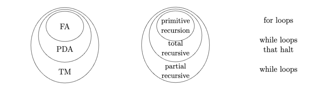
| Function | Loop type | Automaton | Language | Description |
|---|---|---|---|---|
| Primitive recursive | For loops | Finite automaton | Regular language | Regular expression |
| Total recursive | Halting while loops | Pushdown automaton | Context-free language | Context-free grammar |
| Partial recursive | While loops | Turing machine | Turing-recognizable / recursively enumerable | Turing machine description |
It seems feasible that partial recursive functions could be universal. However, we first need to arithmetize the syntax of functions (i.e. describe a way to encode functions as numbers) so that we can pass them to the universal function as input. It is much less trivial to do this for natural numbers than strings.
We define the Gödel numbering function \(g : (\mathbb{N}\to \mathbb{N})\to \mathbb{N}\) that maps a function \(f\) to its Gödel number \(\bar{f}\). These numbers are encoded as powers of prime numbers, i.e. along the prime factor \(\mathbb{N}\to \text{multisets}\) bijection. \(\bar{f}\) is defined as:
I.e. the encoding recursively follows the structures of primitive and partial recursion. Since prime factorizations are unique (fundamental theorem of arithmetic), we can always recover the original structure.
We claim the following:
==What is a configuration of \(f\) on \(x\)? Also, proofs?==
Kleene Normal Form Theorem
TheoremBy corollary, any while loop program can be expressed as a single while loop.
It turns out that for and while loops together form a Turing-complete model computation (1936). So, all programs can be written with just for and while loops (i.e. just with while loops, since a while loop can simulate a for loop).
Mathematical logic employs mechanically checkable reasoning to determine and prove mathematical statements. Different logical systems may be used (commonly, first-order logic), but all logical systems require:
The language of FOL statements can be expressed as a context-free grammar with variables (e.g. \(x\)) and constants (e.g. \(\pi\)) as terminals, and boolean operators (e.g. \(\lnot\)), functions (e.g. \(+\)), relations (e.g. \(=\)), parentheses, and quantifiers (\(\forall, \exists\)) as nonterminal rules and/or parts of nonterminal rules. Thus, every formula is a tree.
A proof in FOL is a finite, directed, tree (maybe a DAG actually?) where vertices are sentences (statements without free variables) and (directed) edges correspond to reasoning rules. An edge joins two sentences when one is derivable from another via a valid reasoning rule. Thus, the leaves of the tree are premises and the root is the conclusion.
Since there are countably many sentences and proof trees, we can enumerate them mechanically to generate a set of provable consequences. This, the language \(C(\Gamma) :=\set{\sigma\mid \Gamma\vdash \sigma}\) is recognizable.
Rules for reasoning are syntactic.
We need to define a way to interpret the strings in our language.
Model
DefinitionGiven a model, the truth or falsity of a FOL sentence is well-defined.
If sentence \(\sigma\) is true under some model \(M\), we denote \(\vDash_M \sigma\). We define the theory \(\text{Th}(M)\) of \(M\) as the language of all statements made true by \(M\), i.e. \(\text{Th}(M):=\set{\sigma\mid \, \vDash_M \sigma}\). Finally, we write \(\Gamma\vDash \sigma\) if we have \(\vDash_M \Gamma\) implies \(\vDash_M \sigma\) under any model \(M\).
With \(\vdash\) and \(\vDash\), we can now describe two properties of logical systems:
Is it possible to find proofs mechanically?
Is there a formal procedure for deciding truth or falsity?
Define model \(A_+\) to be the arithmetic with \(+\), \(\mathbb{N}\) and relations \(<, \leq, =, \geq, >\). Define \(A_{+,\times}\) as \(A_+ \cup \set{\times}\).
\(\text{Th}(A_+)\) is decidable
Theorem\(\text{Th}(A_{+,\times})\) is not decidable, i.e. undecidable
TheoremThis indicates the general result that any system with the capacity to implement/simulate Gödel numbering must inherit undecidability.
Model \(M\) is axiomatizable if there exists set of premises \(\Gamma\) such that \(C(\Gamma)=\text{Th}(M)\), i.e. if we can describe \(M\) as a set of axioms \(\Gamma\).
\(\text{Th}(A_{+,\times})\) is not axiomatizable
TheoremAs a corollary, if we have sound axioms \(\Gamma\subseteq \text{Th}(A_{+,\times})\), then there must exist some \(\sigma\in \text{Th}(A_{+,\times})\) such that \(\sigma\not\in C(\Gamma)\).
Thus far, all terminating problems have been labelled "decidable", but we can reason further about "how long" a decidable program might take to terminate and "how much space" it would use. We've neglected such measures when designing our algorithms, and now we must pay for our sins.
We define the worst-case runtime for Turing machine \(M\) deciding language \(L\) as a function \(t:\mathbb{N}\to \mathbb{N}\) where \(t(n)\) is defined as the maximum number of steps it takes \(M\) to halt on an input string \(w\) of length \(n\).
This definition is concrete, but unnecessarily jagged: the precise definition of \(t(n)\) might be chaotic and categorically difficult to compute. To smooth things out, we partition worst-case runtime functions into classes by their asymptotic efficiency, i.e. their behavior as \(n\to\infty\).
Common Asymptotics Definitions
DefinitionWe have \(f(n)\in o(g(n))\) when for all \(\varepsilon > 0\), there exists some \(n_0<\infty\) such that for all \(n\geq n_0\), we have \(f(n)<\varepsilon\cdot g(n)\), implying \(\displaystyle\lim_{n\to \infty}\dfrac{f(n)}{g(n)}=0\).
The partitioning by the classes \(O\), \(\Omega\), \(o\), \(\omega\) defines an order relations over functions, acting respectively like \(\leq, \geq, <, >\). Partitioning based on \(\Theta\) defines an equivalence relation over functions.
Equivalence of logs: \(O(\log_k{n})=O(\ln{n})\)
Polynomials of a given degree: \(\displaystyle\sum\limits_{i=0}^{d}a_i n^{i}=O(n^{d})\)
Class of polynomial functions: \(2^{O(\log{n})}=n^{O(1)}=\displaystyle\bigcup_{k\in \mathbb{N}}O(n^{k})\). So, \(O(n^k)\subseteq n^{O(1)}\).
Although complexity and efficiently are measured with the same units, they are different things: complexity is a property of a problem, whereas efficiency is a property (namely the worst-case runtime) of an algorithm.
Since complexity is global, we can construct language classes based on complexity. We denote with \(\text{TIME}(t(n))\) the class of languages decidable by a multi-tape (standard) TM in \(O(t(n))\).
Single-tape \(\leftrightarrow\) multi-tape TM
TheoremTo reason about non-deterministic TMs, we amend our definition of \(t\): for ND TMs, \(t(n)\) is the maximum number of steps taken on any computational branch given an input of length \(n\).
Deterministic \(\leftrightarrow\) non-deterministic TM
TheoremThe class \(\mathbf{P}\)
DefinitionWe consider polynomial time to be "reasonable" when designing algorithms, at least compared to exponential time.
When reasoning about problems, by social contract, we assume that structures are encoded in a "reasonable" way, e.g. graphs are adjacency matrices or adjacency lists. We can make a problem trivially easy by picking an "adversarial" encoding. E.g. primality testing is \(O(1)\) (loose bound) if we store numbers as products of prime powers.
Context-free languages are polynomial
TheoremWe prove by describing a polytime algorithm.
Define the problem \(\text{PATH}\) as the language \(\set{\langle G,s,t \rangle\mid G \text{ is a directed graph with path from } s \text{ to } t}\).
\(\text{PATH}\) is in \(P\)
TheoremDefine the problem \(\text{RELPRIME}\) as the language \(\set{\langle x,y \rangle \mid x,y\in \mathbb{N}, \text{GCD}(x,y)=1}\).
\(\text{RELPTIME}\) is in \(P\).
TheoremA verifier \(V\) for language \(L\) is an algorithm (TM) \(V\) such that \(L\) can be defined \(L:=\set{w\mid V\text{ accepts} \langle w,c \rangle \text{ for some } c}\), where \(c\) is a certificate string. \(L\) is polynomially verifiable if \(V\) runs in polynomial time with respect to \(|w|\) (in which case \(V\) is a polynomial time verifier).
The class \(\mathbf{NP}\)
DefinitionWe define the class \(\mathbf{coNP}\) as the class \(\set{L \mid \overline{L}\in\mathbf{NP}}\).
==Note that being in NP is analogous (though not equivalent) to being recognizable. For recognizable \(L\), the recognizer may never halt when \(w\not\in L\) is used as input. However, for \(L\in \mathbf{NP}\), no certificate will exist for \(w\not\in L\), so it can't be verified in polynomial time==.
We define \(\mathbf{NTIME}(t(n))\) as the set of languages decidable in \(O(t(n))\) time by some non-deterministic TM. We can then characterize NP as \(\mathbf{NP}:=\displaystyle\bigcup_{k\in \mathbb{N}}\mathbf{NTIME}(n^{k})\).
Define the problem \(\text{HAMPATH}\) as the language \(\set{\langle G,s,t \rangle\mid G \text{ is a directed graph with a hamiltonian path from } s \text{ to } t}\). Recall that a hamiltonian path visits every vertex exactly once.
Define the problem \(\text{COMPOSITES}\) as the language \(\set{\langle x \rangle\mid x=pq \text{ for } p,q\in \mathbb{N} \text{ where } p,q\ne 1 \text{ and } p,q \ne x}\), i.e. the language consisting of composite numbers.
Define the problem \(\text{CLIQUE}\) as the language \(\left\{ \langle G, k \rangle \mid G \text{ is an undirected graph that contains a clique of size } k \right\}\)
Define the problem \(\text{SUBSET-SUM}\) as the language \(\left\{ \langle S, t \rangle \mid S \text{ is a finite set of integers and some subset of } S \text{ sums to } t \right\}\)
In most of these examples, the corresponding decision problem can't be done in polynomial time because of the search aspect. For example, there are \(2^{|S|}\in O(2^{|S|})\) subsets of a set \(S\), so any decision problem expressible as finding a subset is likely exponential.
Many algorithms proceed by brute-forcing all the possible solutions, then checking them one by one until a valid one is found; it's usually the brute-force step that is super-exponential.
Clearly, \(\mathbf{P}\subseteq\mathbf{NP}\); if a problem can be decided in polynomial time, clearly an instance can be verified in polynomial time. On the other hand, we've yet to find a problem in \(\mathbf{NP}\) that is provably not in \(\mathbf{P}\). The fundamental question \(\mathbf{P}\overset{?}{=} \mathbf{NP}\) remains famously unsolved.
A function \(f : \Sigma^{*}\to \Sigma^{*}\) is polytime-computable if there exists a TM that takes input \(w\), halts with \(f(w)\) written the the tape, and runs in polynomial time with respect to \(|w|\).
Language \(A\) is polytime-reducible to language \(B\), denoted \(A \leq_p B\) iff there exists polytime-computable \(f:A\to B\) such that \(w\in A\) if and only if \(f(w)\in B\).
\(\mathbf{P}\) is closed under polytime reduction
TheoremProblems of satisfiability were among the first problems to be analyzed for complexity, and play a role in defining complexity classes. They are the canonical hard problem.
Define the problem \(\text{SAT}\) as the language \(\set{\langle \varphi \rangle \mid \varphi\text{ is a satisfiable boolean formula}}\), and the problem \(\text{3-SAT}\) as the language \(\set{\langle \varphi \rangle \mid \varphi\text{ is a satisfiable boolean formula in 3-CNF}}\), where \(\text{3-CNF}\) means "in conjunctive normal form, with each clause having \(3\) atoms". It is fairly trivial to see that both problems are in \(\mathbf{NP}\), since booleans formulas can be evaluated in polytime.
\(\text{SAT} \leq_p \text{3-SAT}\)
TheoremWe describe a procedure to convert a boolean formula \(\varphi\) to 3-CNF formula \(\psi\) such that \(\varphi\) is satisfiable if and only if \(\psi\) is satisfiable. For every internal node in \(\varphi\), we add to \(\psi\):
Each time, we encode the operator into multiple clauses by using \(a\) to "bind" the 3CNF clauses together. E.g. for \(\land\), we either have \(a\) or \(\lnot a\), so we either have \(b\land c\) (from clauses \(1\) and \(2\)) for \(a\) or \(\lnot b \lor \lnot c \equiv\lnot(b\land c)\) for \(\lnot a\), as expected. So, \(\psi\) is satisfiable if and only if \(\varphi\) is satisfiable.
\(\text{3-SAT}\leq_p \text{CLIQUE}\)
TheoremWe construct a graph \(G\) from a boolean formula \(\varphi\) as follows:
Then, \(G\) has a \(k\)-clique if and only if \(\varphi\) is satisfiable, since a \(k\)-clique in \(G\) corresponds to a satisfying assignment of \(\varphi\).
This construction is also given in CMPUT 304.
\(\mathbf{NP}\)-Completeness
Definition\(\mathbf{NP}\)-completeness is closed under polytime reduction
TheoremWe also fund that if there exists from \(\mathbf{NP}\)-complete language \(L\) that is also in \(\mathbf{P}\), then we have \(\mathbf{P}=\mathbf{NP}\), since we could reduce any \(\mathbf{NP}\)-complete \(A\) to \(L\in P\).
Cook-Levin Theorem (1971)
TheoremRecall the definition of worst-case time complexity. There is an analogous definition for space: A TM has space complexity \(s(n)\) it never visits more than \(s(n)\) tape cells on input \(|w|<n\). Again, for a nondeterministic TM, no sequence of configurations can visit more than \(s(n)\) spaces.
We have corresponding space complexity classes:
Trivially, \(\text{TIME}(t(n))\subseteq \text{NTIME}(t(n))\) and \(\text{SPACE}(s(n))\subseteq \text{NSPACE}(s(n))\).
Time complexity bound by space complexity
TheoremSpace complexity bound by time complexity
TheoremBasically, space can be reused whereas time cannot.
Savitch's Theorem
TheoremFunction \(t(n) :\mathbb{N}\to \mathbb{N}\) is time-constructible if \(t(n)\geq n\log{n}\) and if the function that maps \(1^{n}\mapsto \text{binary representation of } t(n)\) can be computed in \(O(t(n))\).
Function \(s(n) :\mathbb{N}\to \mathbb{N}\) is space-constructible if \(s(n)\geq \log{n}\) and if the function that maps \(1^{n}\mapsto \text{binary representation of } s(n)\) can be computed in \(O(s(n))\).
These rule out slow-growing functions and uncomputable functions.
Space Hierarchy Theorem
TheoremTime Hierarchy Theorem
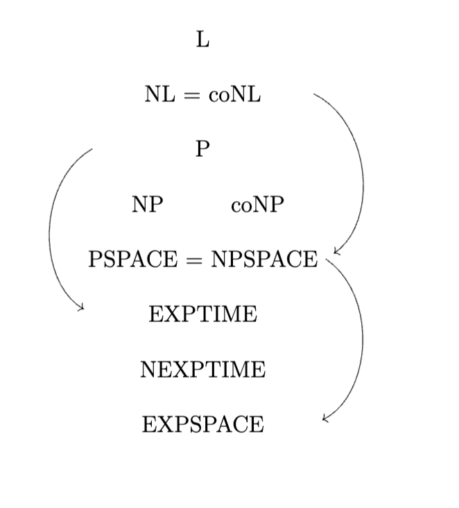
TheoremConcentrically, in order of increasing generality
| Name | Expression | Example |
|---|---|---|
| \(L\) | \(\text{SPACE}(\log{n})\) | \(0^k 1^k\) |
| \(\mathbf{NL}=\mathbf{coNL}\) | \(\text{NSPACE}(\log{n})\) | \(\text{PATH}\) |
| \(P\) | \(\displaystyle\bigcup_{k\in \mathbb{N}}\text{TIME}(n^k)\) | \(A_\text{CFG}\), \(\text{RELPRIME}\), \(\text{CIRCUIT-VALUE}\) |
| \(NP\) or \(coNP\) (not equal!) | \(\displaystyle\bigcup_{k\in \mathbb{N}}\text{NTIME}(n^k)\) | \(\text{SAT}, \text{3-SAT}, \text{CLIQUE}\) |
| \(PSPACE=NPSPACE\) | \(\displaystyle\bigcup_{k\in \mathbb{N}}\text{SPACE}(n^k)\) | \(\text{TQBF}\) |
| \(EXPTIME\) | \(\displaystyle\bigcup_{k\in \mathbb{N}}\text{TIME}(2^{n^k})\) | \(\text{HALT IN }k\), when coded in \(\log{k}\) size |
| \(NEXPTIME\) | \(\displaystyle\bigcup_{k\in \mathbb{N}}\text{NTIME}(2^{n^k})\) | |
| \(EXPSPACE\) | \(\displaystyle\bigcup_{k\in \mathbb{N}}\text{SPACE}(2^{n^k})\) | \(\text{EQ}_{\text{REX}\uparrow}\), i.e. equality for regular expressions with exponents |
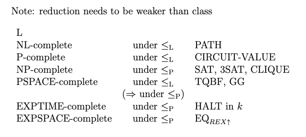
The space complexity equivalent to a polytime reduction is a log space reduction
Log space reduction
DefinitionA log space reduction implies a polytime reduction since \(\text{SPACE}(f(n))\subseteq \text{TIME}(2^{O(f(n))})\)
In turn, a function \(f\) is log space computable if there exists TM with read-only input, write-only output, and working memory that uses \(O(\log{|w|})\) working space to produce \(f(w)\) from \(w\).
We can define completeness for each class we've seen in the same way we defined \(\mathbf{NP}\)-completeness earlier.
Also, it is worth noting which separations we know, i.e. which classes we know are not the same:
All this talk of "compressibility" in the first lecture and we don't cover Kolmogorov complexity? This shall not stand.
prefix vs. prefix-free code
strings are x or w?
In these notes, we reason about the Kolmogorov complexity of strings, but the Kolmogorov complexity of any object with a description language can be reasoned about. E.g. if \(\mathbb{T}\) is the set of all Turing machines, then \(\set{T\in \mathbb{T} \mid \langle T \rangle}\) is the description language of Turing machines (with respect to \(\langle \dots \rangle\)).
random access notes

- depends on a model of computation
- see also: code golf
- prefix-free has to do with nondeterminism? → can nondeterministically compute (?)
- diagonal argument
- bound by actual length of the string → $| \langle M,w \rangle |$
- entropy
Our definitions of time and space complexity describe the behavior of an algorithm while it is running (i.e. at runtime). There is also a notion of complexity the describes how compressible a problem is by considering bounds on the size of the description of an algorithm that solves it.
10101010101010101010101010101010 can be described as "repeat 10 \(16\) times"1001011101101011010001 doesn't have a succinct description like the string above, even though it has more charactersGiven a target string \(x\), consider combinations of Turing machines \(M\) and input strings \(w\) such that \(M\) leaves \(x\) on the tape when run with input \(w\). Thus, \(d:=\langle M,w \rangle\) is a description of \(x\). Let \(\star{d}\) be a minimal description of \(x\) with respect to length.
Then, the plain Kolmogorov complexity \(C(x)\) of string \(x\) is the minimal length \(|\star{d}|\) of a description of \(x\).
By the Church-Turing thesis (and theoretical CS common sense), we can reason about Kolmogorov complexity at a higher level than Turing machines. E.g. K-complexity puts a bound on how succinctly ideas can be expressed with natural language.
There's almost a law of the universe that the first solution you try is almost always the worst one
- CGP Grey
Plain Kolmogorov complexity makes an assumption that it shouldn't: it assumes we know the lengths of strings. This seems reasonable, but becomes a problem when we reason about concatenation. Namely, we can't relate \(C(xy)\) and \(C(x)+C(y)\) without knowing "where to divide \(xy\) into \(x\) and \(y\)". We store the length of strings or use a delimiter, but both of these solutions effectively add characters to the input string.
With plain Kolmogorov complexity, \(C(xy) < C(x)+C(y) + O(1)\) is not generally true as would be expected. We would need a \(O(\min\set{\ln{x},\ln{y}})\) term on the right to balance the inequality.
Prefix-free Kolmogorov complexity solves this problem.
A prefix-free code is a code (in the coding theory sense; here, a subset of \(\set{0,1}^*\)) such that no codeword is a prefix of another. In such a code, we can always determine where a codeword ends, so we don't need to use delimiters or length encoding. A prefix-free Turing machine writes prefix-free codewords (using alphabet \(\set{0,1}\)) to its tape; it is required to read its input exactly once, left to right.
We formally describe the prefix-free Kolmogorov complexity as follows:
The prefix-free Kolmogorov complexity \(K(x)\) of string \(x\) is the shortest prefix-free codephrase that makes Turing machine \(M\) output \(x\), i.e. \(K(x):=\min\set{|w| \mid w\in S^{*}, U(c)=x}\).
A optimal description language is a description language such that any description of an object in an alternate description language can be adapted to the constant language with at most constant overhead. Namely, this constant overhead is a description of the alternate description language.
Invariance Theorem
TheoremRelating plain and prefix-free complexity
TheoremProof: We define the following procedure for converting a basic Turing machine program to a prefix-free Turing machine program:
The description for the prefix-free Turing machine program must include the following:
So, \(K(x)\in O(C(x))\). The precise inequality comes from the encoding scheme we picked for the length of the prefix-free encoding.
Bound on plain complexity relative to length of string
TheoremAs a corollary, we have \(K(x)\leq |x|+2\lg{|x|}\) (from the above-above theorem).
We define the conditional Kolmogorov complexity \(K(x|y)\) of the string \(x\) given \(y\) as the length of the shortest program (in some fixed description language) that outputs \(x\) when given \(y\) as additional input.
For convenience, we will \(K((x,y))\) (i.e. the complexity of the tuple of strings \((x,y)\)) as \(K(x,y)\).
Extra information bound
TheoremProof sketches:
Sub-additivity
TheoremNote that there isn't a way to compare \(K(xy)\) to \(K(x|y)\), \(K(x)\), etc.
Symmetry of Information
TheoremHere, the last equality is proved with a counting argument.
Information non-increase
TheoremNote that we can't compute Kolmogorov complexity by simply enumerating all valid programs and simulating them because not all programs can halt.
Proposition 1: Kolmogorov complexity can get arbitrarily large
PropositionProof: if this weren't true, there would be some \(n\) such that every possible string can be produced by a program expressible with less than \(n\) bits. There are finitely many such programs but infinitely many strings, a contradiction.
Uncomputability of Kolmogorov complexity
TheoremCurrent LLMs make real an interesting thought experiment: code can now be described with natural language. There is an attitude that LLMs make programming "easier" because the programmer must know less to implement their program. However, the results of programs have some (categorically minimal) Kolmogorov complexity, which puts a bound on just how "easy" such programs could be to write. Describing the behavior of a program (as would need to be done to prompt an LLM to write one) cannot be unboundedly easy.
Randomized algorithms and their consequences have been a disaster for my GPA Or they would be, if the science faculty would let me take the damn 499 Shut up and take my money!
implementations of functions with ptimive recursion notes 16
In my (admittedly basic) experience, algebraic structures are described as a tuple of sets and operators defined over those sets, as well as a collection of axioms that describe the behavior of the operators, e.g. a ring is a \(3\)-tuple \((R, +, \cdot)\) where \(+,\cdot\) are binary operators over \(R\) such that [ring axioms]. I've found this structure of description to be a useful constraint for understanding because it forces me to reduce a structure to its essence when describing it this way, much how implementing a program in assembly requires absolute understanding of each internal mechanism. Anyway, this kind of description probably exists in every field of math, but I associate it with algebra the most.↩︎