Provides a unifying method to solve (most) recurrences that occur when evaluating divide and conquer algorithms
Let \(a \geq 1\) and \(b > 1\) be constants, and let \(f(n)\) be a function. Let \(T(n)\) be defined on non-negative integers by the recurrence \[T(n) = aT\left(\frac{n}{b}\right)+ f(n)\]
Then \(T(n)\) has the following bounds
- If \(f(n) \in O(n^{\log_{b} {{a}- \varepsilon}})\) for some \(\varepsilon > 0\) then \(T(n) \in \Theta(n^{\log_{b}{a}})\)
- If \(f(n) \in \Theta(n^{\log_{b}{a}} \times \log^{k}{n})\) for some \(k \geq 0\) then \(T(n) \in \Theta(n^{\log_{b}{a}} \times \log^{k+1} n)\)
- If \(f(n) \in \Omega(n^{\log_{b}{a + \varepsilon}})\) for some constant \(\varepsilon > 0\) and if \(a f\left(\frac{n}{b}\right)\leq \delta f(n)\) for some constant \(\delta < 1\) and all sufficiently large \(n\), then \(T(n) \in \Theta(f(n))\)
Categorizing Recurrences (appendix)
- Top heavy: most of the runtime is found in the initial call
- For \(f(n) = n^{d}, d > \log_{b}{a}\) (case 3 of master theorem)
- Balanced: each level of the tree does about the same amount of work
- For \(f(n) = n^{d}, d = \log_{b}{a}\) (case 2 of master theorem)
- Bottom heavy: most of the runtime comes from the base case (leaves)
- For \(f(n) = n^{d}, d < \log_{b}{a}\) (case 1 of master theorem)
Heaps, Priority Queue, HeapSort (Topic 5)
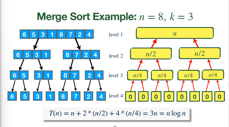
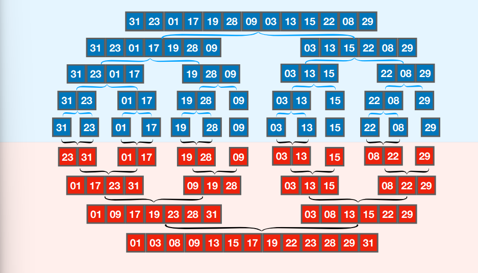
- Recap: Insertion sort is \(\Theta(n^2)\) and Merge sort is \(\Theta(n \log(n))\)
Heaps
- A heap is a binary tree data structure, represented by an array, where the key of the child node is smaller than that of its parent (max heap)
- Max Heap Property: For every node \(j\), we have \(A\left[\lfloor\frac{i}{2}\rfloor\right]\geq A[j]\)
- Thus, the root of the heap is the maximum value
- Min heap: same definition, switch the inequalities from the max heap
- Alternative definition: A heap is a binary tree where every the root of every subheap is the largest value of the subheap
- Heaps are implicit binary trees
- The height of a heap is the number of edges on the longest root-leaf path
- A heap with \(n\) keys has a height \(h = \lfloor \log n \rfloor\)
Array Representation
- The first element of the array is the root; the next two elements are the second layer, the next four are the third layer, etc.
- The intermediate layers are always complete; a heap without the (possibly incomplete) leaf layer is a binary tree
- The leaf layer doesn't need to be complete
Array Indices for Heaps
Definition
- \(\text{leftchild}(A[i]) = A[2i]\)
- \(\text{rightchild}(A[i]) = A[2i+1]\)
- \(\text{parent}(A[i]) = A[\lfloor\frac{i}{2}\rfloor]\)
Almost-Heaps and Max-Heapify
- An almost-heap is a heap where only the root of the heap (might) violate the max-heap property
- The procedure
Max-Heapify(A, i) turns an almost-heap into a heap:
// precondition: Tree rooted at A[i] is an almost-heap
// postcondition: Tree rooted at A[i] is a heap

lc = leftchild(i), rc = rightchild(i), largest = i;

//finds the largest child of A[i] (either left or right)
if(lc <= heapsize(A) && A[lc] > A[largest]) {
    largest = lc
} //else?
if(rc <= heapsize(A) && A[rc] > A[largest]) {
    largest = rc
}

//if the root is not in the right spot, it switches it it with
//the largest child, then recursively calls Max-Heapify
//on that child's subheap
if(largest != i) {
    swap(A[i], A[largest])
    Max-Heapify(A, largest)
}
Running Time
- We find the running time of
Max-Heapify is \(O(h) = O(\log(n))\), since it gets run once per layer of the heap
- We can also find this since \(T(n) \leq T\left(\frac{2n}{3}\right)+ c\) ??
Building a Heap
Procedure
- Each leaf node is a key in and of itself, since it follows the max-heap property
- Thus, the nodes on the second-bottom layer are almost-heaps, since both of their children are the roots of heaps
- We use
Max-Heapify to turn them into heaps
- Now, the nodes on the third level are almost-heaps because we turned their children into heaps. We can also
Max-Heapify this into heaps
- Keep repeating this process recursively up the tree
- The whole tree becomes a heap
Pseudocode
- The procedure can be expressed using the following pseudocode
let i = floor(length(A)/2);

for (i downto 1) {
    Max-Heapify(A, i)
}
- Note that we simply perform
Max-Heapify on the first half of the array
- Since this is where all the non-leaf nodes are stored (and the leaf notes are heaps already), this works
Running Time (loose)
- The running time of
Build-Max-Heap is \(\dfrac{n}{2} \times c \times \log(n) \in O(n \log(n))\)
- \(\frac{n}{2}\) is the number of times
Max-Heapify(A, i) is called
- \(c \times \log(n)\) is the running time we determined for
Max-Heapify
- Note that \(O(n\log(n))\) is not tight
- This assumes the worst case running time (\(c \times \log{n}\)) is the same for all the nodes; this actually depends on their height
Running Time (tight)
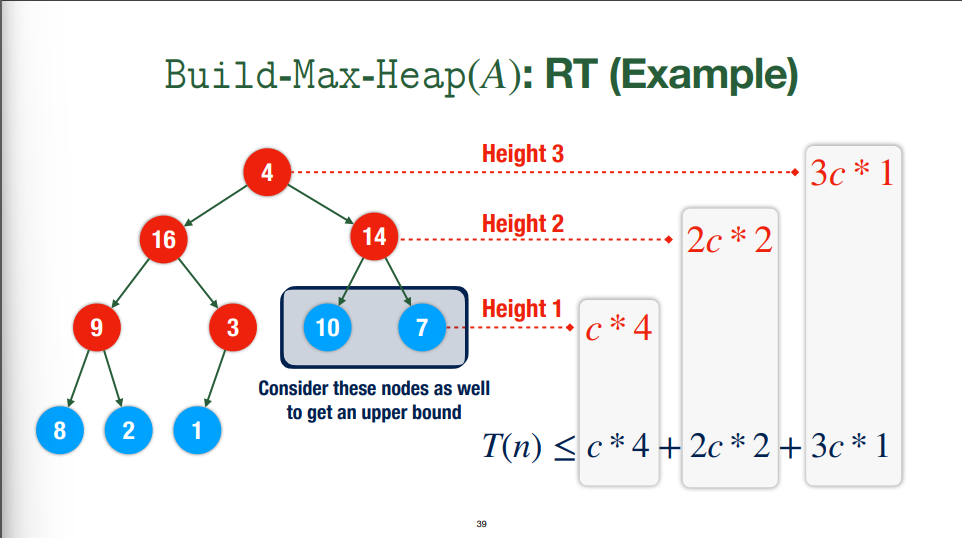 - $c$ is the worst case running time for `max-heapify` on a tree with a root and two leaves (it's constant)
- To find the WC runtime of each layer, we take $\text{number of nodes in the layer} \times \text{number of layers below node} \times c$
- We need to sum all of these to get the RT for the whole algorithm
- Height: $k = \lfloor \log{n} \rfloor$
- Base of tree ($k=0$): at most $2^{\lfloor \log{n} \rfloor}$
- Number of nodes: $2^n$
- For an $n$-element heap, the maximum number of elements of height $k$ is $\dfrac{n}{2^k}$
- So: $\displaystyle\sum\limits_{k=1}^{\log{n}} kc \times \dfrac{n}{2^{k}}\geq T(n)$
- We can use algebra to find that is this $O(n)$ (i.e. reduces to a constant times $n$)
- Another way to look at it: $T(n) \leq \displaystyle\sum\limits_{k=1}^{\log{n}} kc \times \dfrac{n}{2^{k}} \leq nc \sum\limits_{k=1}^{\infty}\dfrac{k}{2^k}$. Note that $\displaystyle\sum\limits_{k=1}^{\infty}\dfrac{k}{2^{k}} \leq \int^{\infty}_{0}\dfrac{x}{2^{x}} \, dx$, which is constant
- $c$ is the worst case running time for `max-heapify` on a tree with a root and two leaves (it's constant)
- To find the WC runtime of each layer, we take $\text{number of nodes in the layer} \times \text{number of layers below node} \times c$
- We need to sum all of these to get the RT for the whole algorithm
- Height: $k = \lfloor \log{n} \rfloor$
- Base of tree ($k=0$): at most $2^{\lfloor \log{n} \rfloor}$
- Number of nodes: $2^n$
- For an $n$-element heap, the maximum number of elements of height $k$ is $\dfrac{n}{2^k}$
- So: $\displaystyle\sum\limits_{k=1}^{\log{n}} kc \times \dfrac{n}{2^{k}}\geq T(n)$
- We can use algebra to find that is this $O(n)$ (i.e. reduces to a constant times $n$)
- Another way to look at it: $T(n) \leq \displaystyle\sum\limits_{k=1}^{\log{n}} kc \times \dfrac{n}{2^{k}} \leq nc \sum\limits_{k=1}^{\infty}\dfrac{k}{2^k}$. Note that $\displaystyle\sum\limits_{k=1}^{\infty}\dfrac{k}{2^{k}} \leq \int^{\infty}_{0}\dfrac{x}{2^{x}} \, dx$, which is constant
Priority Queues
Definition and Motivation
- An abstract data structure for maintaining a set \(S\) of elements, each of which has a key that represents the priority of the element
- An element with a given priority can be added
- When an element is removed, it must be the element with the highest priority
- Operations usually supported:
initialize (keys), maximum, exract maximum, increase (key), insert (key)
Heap Implementation
initialize (keys): use build-max-heap to structure the array into a heapmaximum: the maximum element is already at the top of the heap, i.e. \(A[1]\). Simply return thatextract-maximum: return the max value from the top of the heap. Place the last element of the heap at the top of the heap (i.e. reduce the heap size by 1, copy the value to \(A[1]\)). Then run max-heapify to turn the resulting structure into a heap again and return the max.
- This is \(O(\log{n})\) due to
max-heapify
increase (key): increase the value of the key. If the key is now larger than its parent, move it up and check again. Stop when this is not the case or the key is at the top of the heap
- Inverse of max-heapify
- This is also \(O(\log{n})\)
heap insert (key): increase the size of the heap and add a key at the bottom (value can be anything smaller than the intended key, e.g. \(-\infty\)). Then, run increase with the intended value
- This is obviously \(O(\log{n})\) like
increase
- For decreasing a key, we can change the key and then call
max-heapify on the subheap where the key is the root, since it will be an almost-heap
Heapsort
Motivation and Implementation Sketch
- Heaps can be used to design a sorting algorithm: Heapsort
- General idea
- Build an array into a heap: \(\Theta(n)\)
- \(A[1]\) is the maximum, so should be at the least position
- Switch \(A[1]\) and \(A[n]\) and decrease the heap size by \(1\), since \(A[n]\) is now in the correct position
max-heapify the unsorted part of the array, i.e. \(A[1\dots (n-1)]\), which is an almost-heap- Keep repeating these steps to fill positions \(n-1\), \(n-2\), etc.
Runtime
- We know
build-max-heap is \(\Theta(n)\)
- Informal: we know running
max-heapify on each element of the array is \(O(n \log{n})\)
- Formal: \(\displaystyle \sum\limits_{i=2}^{n} \log{i} \geq \sum\limits_{i=\lceil \frac{n}{2} \rceil}^{n} \log{\frac{n}{2}} = \lfloor \frac{n}{2}\rfloor \times (\log{n} - 1) \geq \frac{1}{3}n\log{n}\), so we know that this process is also \(\Omega(n \log{n})\)
- Therefore, heapsort has a runtime of \(\Theta(n \log{n})\)
Quicksort, Sorting Lower Bound BST, Balanced BST, Hash Table (Topic 6)
Quicksort
- Quicksort overview: Divide the array into two subarrays around a pivot such that everything before the pivot is smaller than it and everything after it is larger. Then recursively quicksort each half. Finally, each half is combined, which is trivial since quicksort is sorted in place
- Uses the divide and conquer paradigm
Pseudocode
QuickSort(A, p, r):
    // sorts A = [p ... r]
    if(p < r) {
        // A[q] is the pivot
        // all elements before q are smaller, all after are larger
        // note: partition both modifies A (side effect) AND returns q
        q = Partition(A, p, r)
        // recursive calls
        QuickSort(A, p, q-1)
        QuickSort(A, q+1, r)
    }

// Partition subprocedure
Partition(A, p, r):
    // last element of array being examined is picked as a pivot
    pivot = A[r];
    // "switch counter" (i is an index; counts up from start index)
    i = p-1
    for(j from p to r-1) { // counts up from start to second last element
        // if current element is smaller than pivot, switch and increment counter
        if(A[j] <= pivot) {
            i = i+1;
            swap(A[i], A[j])
        }
    }
    // switch last element and element in the "pivot spot", as determined by
    // incrementing i
    // note that we compared with r when switching and incrementing, so this
    // is why we can simply swap these and know the list is in the right form
    swap(A[i+1], A[r])
    return i+1
Partition Explanation
- The pivot is \(A[r]\)
- Looks at the keys of the array from \(p\) to \(r-1\)
- \(j\) is the current element we are considering
- \(i\) is the index of the last known element that is smaller than or equal to the pivot
Runtime
- Quicksort is useful to analyze because is provides a good model for analyzing algorithms, as well as because it shows how useful randomization can be
Recursion Tree
- The recursion tree for quicksort isn't deterministic; it will be of different depth and balance depending on the distribution of the input
- To form the recursion tree, the root is the pivot and the children are the first and second recursive calls
- Since the keys in the left subtree are less than the pivot and those on the right are larger, the quicksort recursion tree is a binary search tree
Recurrence
- For \(n \geq 1\), \(T(n) = 0\) since there is only a pivot, so the algorithm takes constant time
- Otherwise, we have \(T(n) = T(n_{1}) + T(n-1-n_{1}) + (n-1)\)
- \(T(n_1)\) is the recursive call for the list less than the pivot; we say is has \(n_1\) elements since we won't know how many it will have
- Thus, the other recursive call is \(T(n-1-n_{1})\) since the pivot isn't part of it
- \((n-1)\) since the pivot is compared with every other key
Worst-case
- Notice that when both recursive subarrays are non-empty, there are \(n-3\) comparisons in the level below the one with \(n\) comparisons: \((n_{1}-1) + (n-1-n_{1}-1) = n-3\)
- However, when one is empty, there are \(n-2\) key comparisons, since one side is the \(T(0)\) case of the recurrence
- Solving the recurrence (using the worst-case insight below) by iterated substitution shows that \(\boxed{T(n) \in \Theta(n^2)}\)
- Note that the absolute worst-case running time is when the list is sorted in reverse-order, since the pivot moves one spot each time and always leaves an empty subarray
- In this case, quicksort devolves into insertion sort
Best-case
- The best case for quicksort is when the tree is as balanced as possible, i.e. the list is sorted in ascending order
- Every partition is a bipartition: the array is always split in half
- For this case, the recurrence it \(T(n) = 2 \times T\left(\dfrac{n-1}{2}\right)+ (n+1)\), since \(n_{1} = \dfrac{n-1}{2}\)
- Using the master theorem shows that this \(\boxed{T(n) \in \Theta(n \log{n})}\)
Average Case
- However, this running time is common because it happens any time the split of the array is a constant proportion, even if it's not \(\frac{1}{2}\)
- I.e. \(T(n) = T(q \times n) + T((1-q)\times n) + cn\) for \(q \in \mathbb{Q}\) can be shown to lead to \(O(n \log{n}) \implies \Theta(n \log{n})\)
- We assume each possible input has equal probability, i.e. \(n_{1}\sim \mathcal{U}(0, n-1)\); each \(n_{1}\in \set{0, 1, \dots n-2, n-1}\) has probability \(\dfrac{1}{n}\) of being chosen
- So, \(T(n) = (n-1) + \dfrac{1}{n}(T(0) + T(n-1)) + \dfrac{1}{n}(T(1) + T(n-2)) + \dots + \dfrac{1}{n}(T(n-1) + T(0))\) since each value of \(n_1\) has equal probability \(\dfrac{1}{n}\). This reduces to \(\displaystyle \dots = (n-1) + \dfrac{2}{n} \sum\limits_{i=0}^{n-1} T(i)\), ==which implies \(\Theta(n \log{n})\) somehow?==
Storage
- Unlike mergesort, quicksort sorts in place: no extra space is required to perform the sorting algorithm
- Mergesort uses \(\Theta(n)\) extra space since a new list worth of space is required
- Quicksort only uses \(\Theta(1)\) since the amount of space required is the same, no matter the size of the list
Random Quicksort
- Instead of using
Partition, we invoke a function RandomPartition that randomly chooses an integer \(p \geq i \geq r\) and swaps \(A[i]\) with \(A[r]\), then calls Partition(A, p, r)
- This effectively chooses a random pivot from the list
- This essentially guarantees the expected worst-case running time to be \(\Theta(n \log{n})\)
Notes on Randomness
- For average case analysis, we make an assumption about the input, i.e. that any instance is equally probable
- This may not hold in an actual program; we are making assumptions that input is random, which we can't guarantee
- For randomized algorithms though, we can guarantee the randomness will occur because it is baked into the algorithm itself
- So, since the random case always happens, we can use it when conducting worst-case analyses
- In a deterministic algorithm, there is no randomness, so the same output always yields the same calculations
- In a randomized algorithm, the same input always maps to the same output, but the calculations involved may be different
- These are often implemented to improve the worst-case performance
Lower Bound for Sorting
- Lower bound for a specific problem: \(\forall \text{ algorithm } A, \exists \text{ input } I \text{ such that } \text{runtime}(A(I)) \geq \dots\), i.e. for every possible algorithm that solves the problem, the runtime will be at least the lower bound
- We prove lower bounds by constructing ("difficult") instances of a problem that have the longest runtimes
- All the algorithms we've looked at so far are \(\geq \Theta(n \log{n})\). It turns out that no sorting algorithm has a lower bound less than \(\Theta(n \log{n})\)
- I.e. \(\text{runtime}(A(I)) \geq c \times n\log{n} + o(n \log{n})\)
Useful Trees
Recursion Tree
- Each node corresponds to a recursive call; the whole tree corresponds to an algorithm execution
- Describes an algorithm execution for one particular input by showing each recursive call
- Why it's helpful: the sum of the operations over all the nodes is the total number of operations for the algorithm execution
Decision Tree
- Each node corresponds to an algorithm decision
- Describes the algorithm execution for all possible inputs by showing all possible decisions
- A single algorithm execution corresponds to a root-to-leaf path
- Why it's helpful: sum of the numbers of operations over nodes on one path is corresponds to a particular instance of the algorithm; all instances (i.e. every possible result) exist in the tree
Showing a Sorting LB with Decision Trees
- Comparison-based sorting algorithms have binary decision trees
- There are at least \(n!\) leaves, which correspond to the \(n!\) sorted arrays of size \(n\) that can possibly exist
- Thus, the tree must have at least \(1 + \log{n!}\) levels, since this is the minimum number of levels in a binary tree with \(n!\) nodes
- So, a longest root to leaf path is at least \(n!\)
- Therefore, in the worst case, an algorithm makes \(\log{n!} \in \Theta(n \log{n})\) comparisons
Dynamic Sizes
- So far, everything we've been sorting on is of static size
- However, it's also worth studying algorithms and data structures in the dynamic case, i.e. when the size of the array is not fixed
- Options:
- Use a data structure that does insertion and deletion quickly (array, list, hash table) and run a sorting algorithm when required
- Use a data structure that keeps elements sorted (e.g. BST)
Binary Search Trees (BSTs)
Tree Terms
- A rooted tree is a data structure where each child has a unique and distinct pointer to another rooted tree
- It has a single root node
- Descendant: \(u\) is a descendant of \(v\) if a path of child pointers from \(v\) to \(u\) exists
- Leaf: a node with no children
- Binary rooted tree: A rooted tree where each node has at most two children
- Height: number of edges in the longest root-leaf path in the tree
- Layer<\(i\)>: the set of nodes with distance \(i\) from the root
Binary Search Tree Definition
- Binary Search Tree: a rooted binary tree where every node \(v\) has the following properties
- All keys in the left subtree of \(v\) are smaller than \(v\)'s key
- All keys in the right subtree of \(v\) are larger then \(v\)'s key
- A BST with \(n\) nodes may have heights of up to \(h \approx n\) in the worst case
Binary Tree Operations
- Search: we check if our key is equal to that of the node we are checking. If it's smaller, we recurse on the left subtree, otherwise the right.
- Runtime: \(O(h)\), since this is executed once for each layer of the tree
- Delete: if the node is a leaf, we remove it. Otherwise, we take the largest element of the "smaller than" subtree and make that the node node at the location we are deleting from
- Also \(O(h)\) runtime for the same reason
- Outputting sorted sequence: Recursively to this to left subtree, print the current key, recursively do this to the right subtree
- \(O(n)\) because, by definition, we print each element once
AVL Trees (Balancing BSTs)
- Note that if a binary tree is "balanced", \(h \approx \log{n}\) so both search and insert/delete are \(O(\log{n})\), which overall is better than both arrays and linked lists, which is massively helpful
- So, we need a way to keep BSTs balanced
AVL Rotations
- Key operation: rotations
- Right-rotate: the old root becomes the right child of the new root
- Left-rotate: the old root becomes the left child of the new root
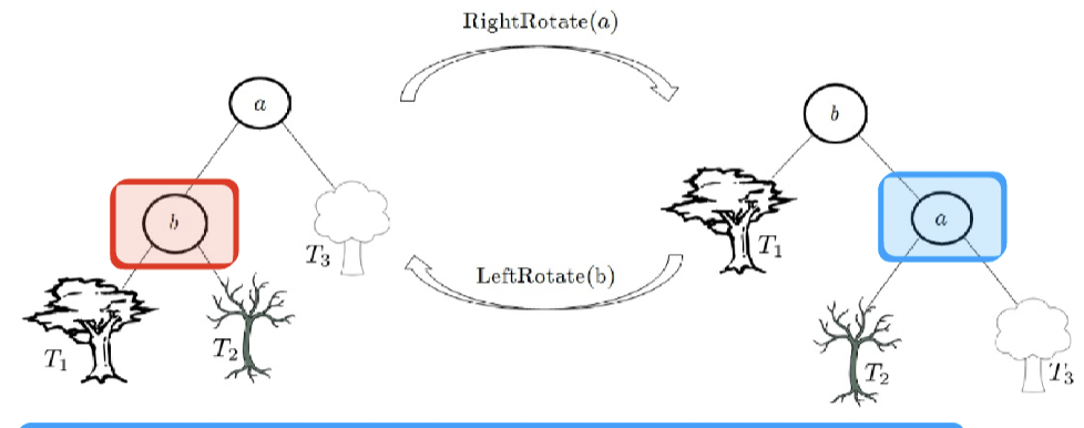
- Both of these are trivially \(O(1)\)
AVL Tree Definition
- An AVL tree is a BST where, for any node, we have \(|h_L - h_R| \leq 1\), I.e. the heights of both subtrees are as close as possible
- An AVL tree with height \(h\) has at least \(Fib(h)\) nodes
- This can be derived from the AVL tree property above, assuming that (WLOG) each right subtree has one more layer than the left one
Maintaining the AVL Property
- Four cases for balancing the BST: single rotation (cases 1 and 2), double rotation (cases 1 and 2)
- more detail here
- Essentially, if a subtree is unbalanced, there is a way (one of the four) to reorder the nodes so that it is indeed balanced
Hash Tables
- AVL trees have \(O(\log{n})\) search and insert/delete, but we can do better for average-case; we can get both as low as \(O(1)\) with hash tables
Hash Table Definition
- We have an array \(T\) of size \(m\) and some hash function \(h : U_k \to \set{0, 1 \dots m-1}\), where \(U_k\) is the set of keys we wish to store. When inserted, each key \(k_i\) is stored at \(T[h(k_i)]\)
- Collisions (I.e. multiple keys mapping to the same number) are resolved by chaining the keys together in a doubly linked list starting at the space in \(T\) where they are mapped
- Insertion, search, and removal are all done by finding the corresponding address in the table, going to it, then searching through the linked list
Hash Table Runtime
- Insert and Delete can both be done in \(O(1)\) with doubly linked lists
- The running time of search is dominated by the longest chained list; in the worst case, it is \(O(n)\), since all the keys can theoretically be mapped to the same location
- Define \(\alpha = \dfrac{n}{m}\) as the average number of elements per slot in the hash table (load factor)
Types of Hashing
- If hashing Is uniform (I.e. any slot is equally likely), then the load factor is constant; so search is \(O(1)\) since it is dominated by the load factor
- E.g. an unsuccessful search takes \(O(1+\alpha )\)
- Universal hashing: a set of hash functions is universal if the probability of any two functions hashing to the same value is less than \(\frac{1}{m}\)
- If we randomize the hash functions at runtime, any sequence of operations generally has a good average-case runtime
- Example set of uniform hash functions: for a random prime \(p > |U|\) and random \(a, b\) from \(\set{0_b , 1, 2, \dots p-1}\), we define \(h_{ab}(k) = ((a \times k + b)\mod{p}) \mod{m}\)
Greedy Methods (Topic 7)
Greedy Algorithms
Always make choices that look best at the current step. These choices are final and cannot be changed later
- Useful for optimization problems, where we are trying maximize or minimize something
- Greedy algorithms are generally easy to come up with, but hard to prove correct (I.e. optimal)
Optimization Problems
- General statement: Choose some \(x\) (decision variable) where \(x \in C\) (feasible region) such that \(f(x)\) (objective function) is minimized
- \(\star{x}\) is the optimal decision and \(f(\star{x})\) is the optimal value
- Are useful in transportation, logistics, internet infrastructure, economics, ML (e.g. supervised learning, deep learning, reinforcement learning)
- Optimal solutions may be unique or non-unique (I.e. multiple instance of an optimal solution)
Proof Strategy
- We want to show that each greedy choice can replace some portion of the optimal solution, such that this altered new solution is still optimal
- This is done one item at a time
- unified description here
Properties of Greedy Solutions
- Substitution property: Any optimal decision can be altered to become our greedy choices without changing its optimality (also called the greedy choice property in CLRS)
- We can prove correctness by showing this holds
- Optimal Substructure Property: the optimal solution contains optimal solutions to subproblems that look like the original problem
- This property is key to dynamic programming
- For greedy algorithms, the substructure is the rest of the choices we have to make (?)
- Greedy algorithms stay ahead: after each step, their solution is at least as good as any other algorithm's
- Greedy algorithms make a myopic (locally optimal) sequence of decisions
Fractional Knapsack Problem
- Suppose we have a set \(S\) of \(n\) items, each with value \(b_i\) and weight \(w_i\). We have a knapsack (bag) which has a weight capacity \(W\). We can pick each item at a fraction, I.e. we can pick as much of it as we want up to the amount of it we have. What is the maximum profit we can carry in the knapsack?
- Formally, we wish to maximize \(\sum\limits_{i=1}^{n} s_i \times \frac{b_i}{w_i}\) where \(\sum\limits_{i=1}^{n} s_i\leq W\) and \(0 \leq x_i\leq w_i\) for all \(i\)
- Greedy approach: start by picking the item with the highest value/weight ratio one at a time
- Implementation: we must sort the set of items \(S\) by this ratio (\(\Theta(n \log{n})\))
Intuition/Proof
- The first choice is saturated if we have run out of choices for it
- We always know. by definition, that \(profit(\star{s}) \geq profit(s)\) for any \(s\)
- We proceed by showing the first item is saturated, then the second, etc.
- Claim 1: there is an optimal solution where item 1 is saturated. For the optimal solution, either
- Item 1 is indeed saturated, so we are done
- Item 1 is not saturated.
- Case 1: knapsack is not full (I.e. we are able to put some of it in the knapsack). So, since item 1 is the most valuable, the solution where we take as much of it as we can cannot be smaller than the optimal solution
- Case 2: Knapsack is full. Then, there must be some of the item in there because replacing the space it takes with a different (less valuable) item would decrease the cost
- add formal math stuff here later
- This argument can be repeated for each most valuable item (I.e. when the most valuable item is used up, we apply to the second most valuable, etc)
Job Scheduling Problem
- Instance example: we have a bunch of classes at specific times. How can we schedule the classes such that the least number of rooms as possible are used?
- Formal: we have a set \(T\) of \(n\) jobs, with start and finish times \(s_i\) and \(f_i\)
- ESTF: Earliest-start-time-first
- First, we sort all the jobs by start time
- Then, we start adding jobs in order, each on a new machine
- Each time a job gets added, its end-time gets added to a min-heap, so the closest end time is always on top. Before a job gets added to a new machine, we check the min-heap to see if the closest job has finished. If so, we start the new job on that machine instead (and add and remove from the min heap appropriately)
- ESTF can be shown to be optimal by considering that we can always find a set of \(k\) jobs running simultaneously if \(k\) processors are being used. Thus, it is impossible for the jobs to be scheduled on \(k-1\) processors (and thus it is optimal).
Activity Selection
- Instance example: the are various classes happening throughout the day. What is the largest subset of non-conflicting classes that one student can fully attend.
- ESTF won't work here, nor will shortest first
- Solution: Earliest finish time first (EFTF)
- Optimality proof: we show our decisions are correct by showing that there is an optimum schedule that contains everything we have selected (so far) and has omitted everything we have decided to omit (so far)
- I.e. there is an optimal schedule that looks like what our algorithms is doing so far
- This is proven with induction
Divide-and-Conquer Revisited (Topic 8)
- For many algorithms, applying divide and conquer is the first step. The next is to figure out how to reduce the number of recursive calls
- The coefficient of \(T(f(n))\) has large performance implications
Exponentiation
- For \(b, n \in \mathbb{N}\), we wish to compute \(b^n\)
- This has many practical applications for large \(n\), e.g. cryptography
- Naive approach I: use a for-loop to multiply \(b\) by itself \(n\) times (\(O(n)\))
- Naive approach II: just divide and conquer by splitting the problem in half each time (also \(O(n)\))
- Improvement: for even \(n\), we can reduce the number of recursive calls by saving the result of \(\exp(b, \frac{n}{2})\) and squaring it. For odd \(n\), we simply call \(\exp(b, n-1)\) so that we have an even recursive call next time
- Note: when I tried to derive this algorithm on the test (yikes), it didn't occur to me that I was making the same recursive call twice when I could just square it
- We can show that this ends up being \(O(\log{n})\) since we end up making at most one recursive call per things, and since each (even) recursive call divides the problem in half (and there is at most one odd call before it), the problem gets divided in half each time*
Karatsuba's Algorithm for Large Integer Multiplication
- Regular "elementary school" multiplication takes \(O(n^2)\)
- Naive divide and conquer: we take a four digit number and express it as four two digit multiplications, where we multiply by powers of the base and perform remaining multiplications recursively
- This is also \(O(n^2)\), since there are four recursive calls with inputs that are half as big as the original
- Karatsuba is like divide and conquer, but is slightly more efficient with its recursive calls
- We have \(I = w \times x\) and \(J = y \times z\)
- So, \(I \times J = w \times y \times 2^{n}+ (w\times z + x\times y) + x\times z\)
- Let \(p = w\times y\) and \(q = x\times z\), and \(r = w\times z + x\times y\)
- Notice that \((w\times z + x\times y) = r-p-q\), which requires one less multiplication to compute
- So, if we compute and then store \(p\), \(q\), and \(r\), then calculate \(r-p-q\), we perform the recursive step in 3 multiplications instead of 4
- So, the run time is \(O(n^{\log_{2}{3}}) \in o(n^2)\)
- The \(2^n\) multiplications can be accomplished with \(O(1)\) shifts and we assume addition is \(O(1)\), so the \(f(n)\) term does not dominate
Strassen Matrix Multiplication
- Regular algorithm: traverse each row of \(X\) and each column of \(Y\) (\(n^2\) choices) and compute the \(O(n)\) product for each coordinate, so \(O(n^3)\)
- Naive divide and conquer: divide each matrix into four quadrants, then perform the required matrix multiplication and addition. Turns out that this is also \(O(n^3)\)
- Strassen: found 7 matrices (that each take one matrix multiplication to calculate) that can be combined together with multiplication and subtraction in order to form the desired matrix product
- So, the runtime is \(O(2^{\log_2{7}})\)
Summary
- When writing divide and conquer algorithms, we should look for opportunities to reduce the number of recursive calls at each step, as this will improve performance significantly as inputs get larger
- These often come at the expense of non-recursive operations
- In particular, see if any of the recursive calls can be computed into one of the other recursive calls without using constant time operations (or any operation more efficient than the recursive option)
Dynamic Programming (Topic 9)
Problems are solved recursively, but the results of individual recursive calls are saved and may be re-used
Divide and Conquer vs. DP
- Divide and Conquer: We take a big problem, divide it into multiple subproblems, solve those, then re-integrate those into the full solution
- Each of these subproblems are independent of each other, and each subproblem relates only to its parent
- For dynamic programming, there may be more complex (but still bottom-up) relationships between subproblems
- Subproblems may be shared, i.e. have multiple parents
- They may also have varying numbers of children
Example: Fibonacci
- Regular algorithm makes wayyyyy too many recursive calls with values that have been computed before
- DP approach: each time we calculate a value, add it to an array like \(A[n] = fib(n)\). Then, when evaluating a (likely recursive)
fib call, retrieve the value from the array if it's there, instead of calculating it.
- This is \(\Theta(n)\) time and space, instead of \(\Theta\left(\left( \dfrac{1+\sqrt{5}}{2}\right)^n\right)\) time
Properties of DP Solutions
- Overlapping subproblems: different branches of recursive calls complete each other's work (repetition)
- Optimal substructure: the optimal solution for the overarching problem is dependant only on the optimal solutions for subproblems (dependency)
- The subproblems should be able to be evaluated in polynomial time
- Types of ways to go about writing a DP solution
- Tabulation: Bottom-up approach to DP algorithms. Before solving a subproblem, we must solve its subproblems first
- Memoization: Top-down approach to DP (can be refactored into this)
- Informal: the running time is (or is clearly derived from) the number of possible filled spaces in the lookup table
General Steps for DP
- Find a recurrence relation for the problem
- Check if the recurrence ever makes any of the same calls, and if there are reasonable amount of different ones
- What is the dependency among subproblems
- Describe array (or I guess any data structure) of values that you wish to compute. Each value will be the result of a specific recursive call
- Fill the array from the bottom up* (backward induction). Solutions to subproblems will be looked up from the array instead of being computed themselves
- Bottom up: loop over all the values up to the one we want, and fill in the array slot for each value looped over. This means we don't have to check if something is in the array because we know it will be
- Can also be done top-down (i.e. checking and calculating if it's not there)
Integral Knapsack Problem
- Like the fractional knapsack problem, but fractions of items can be taken
Naive Recursive Solution
- For each item \(v\), we calculate the following recursive calls
- Take the item: recursive knapsack on \(W - w_i\) and the set of items without \(v\)
- Leave the item: recursive knapsack on \(W\) and the set of items without \(v\)
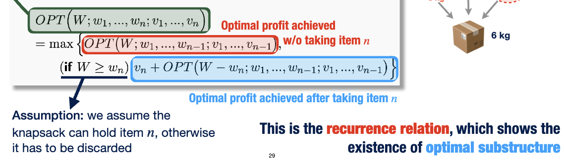
- Recurrence relation (formal): \(OPT(W; w_1 \dots w_n; v_1 \dots v_n) = \max{\set{OPT(W; w_1 \dots w_{n-1}; v_1 \dots v_{n-1}), v_n + OPT(W - w_n; w_1 \dots w_{n-1}; v_1 \dots v_{n-1})}}\)
- First term in the \(\max\) is not choosing the item, the second one is choosing it
Applying DP
- There are indeed repeated subproblems; they exist when the same remaining space is calculated with the same set of available items
- So, we can create a table with "remaining capacity" on one axis and "first \(n\) items" on the other, since items are always evaluated in the same order
- This contains all possible sets of items that we could have looked at already
- Any possible recursive call we can make has a space in the table, so we can look to see if anything is there first and only evaluate a recursive call if there isn't anything
- The overall runtime is \(O(nW)\)
- This is the number of spaces in our table; this is the most amount of computations that need to be done (the individual check for each is \(O(1)\))
Better Solution: Working Bottom-up
- We can fill in our table in the following way before we even run our algorithm
- If we've looked at \(0\) items so far, our optimal profit for those is obviously \(0\), no matter our remaining capacity, so we can fill the whole first row with \(0\)s
- Next row (1): anything below the weight of our first item will take the value from the previous row (in this case 0), because there must be enough capacity left to hold it. Everything else in the row will be the item in the previous row plus the value of the item
- Next row (2): anything below the weight of the third item is still 0. If the weight of the third item is \(w\), we look at the item \(w\) cells to the left in the row above to figure out what to do. If we can add the current item to the knapsack, we do (and get the new total value). Otherwise, the value of a cell is the same as the cell above it
- Idea: for row \(n\) (i.e. first \(n\) items looked at), if the \(n\)th item was height \(w\), we look \(w\) cells to the left in row \(n-1\). If that cell exists (not off the side of the table) and the sum of that cell and the current value is larger than the value in the cell above the one we look at, we put that sum in the cell (corresponds to putting that item in the knapsack). Otherwise, we put the value above in there (corresponds to not putting it in the knapsack)
Rod Cutting Problem
- We have a length of rod to sell, and the price of a piece of length \(i\) is \(p_i\). How do we maximize the profit we can get by selling our rod?
- Naive solution: try all possible combinations (\(O(2^n)\)) since we have \(n-1\) places in the rod that can be either cut or not
- Recursive solution: we cut the rod once (\(n-1\) different ways to do this). The solution is the max of the sum of the optimal ways to cut each of the two subrods (this is called recursively)
- DP solution: we keep track of the optimal value of each length in an array, and add to it each time we calculate a new value.
- Bottom up (tabulated): we loop \(k\) from 1 to \(n\) and calculate the optimal value for length \(k\) each time.
- Top-down (memoized, requires helper function): essentially: we make an array to store values and call the function recursively, looping over every length possible with one cut.
- Runtime: \(O(n^2)\), since we have to fill \(n\) cells and that calculation is \(O(n)\) itself
Longest Common Subsequences
- Subsequence: any subset (not necessarily contiguous) of a sequence/array
- Recurrence: \(LCS(x_1 \dots x_n; y_1 \dots y_m) = \max{\set{LCS(x_1 \dots x_{n-1}; y_1 \dots y_m), LCS(x_1 \dots x_{n}; y_1 \dots y_{m-1}), 1 + LCS(x_1 \dots x_{n-1}; y_1 \dots y_{m-1})}}\)
- First two cases: we skip a character (first \(x\), second \(y\))
- Last case: we match a character
- Table: one axis is all the possible "states of consideration" of the first string (the contiguous blocks of 1, 2, 3, etc characters that we have examined, starting from the first one), the other axis is that of the second string
- Then our "recurrence" becomes \(D[i, j] = \max{\set{D[i-1, j], D[i, j-l], 1 + D[i-1, j-1]}}\)
- The DP solutions (top-down and bottom-up) use this table to stop repeated calculations
- Runtime is \(O(n + m + mn)\) because we have to fill the table (\(mn\) cells)
Graphs, BFS, DFS (Topic 10)
Graph Terms
- Nodes/vertices \(V\): a set of \(n\) elements with unique identifiers, usually numbers in \(\set{1, 2, \dots, n}\)
- Edges \(E\): set of unordered or ordered (directional) connections between nodes in a graph
- Undirected: each edge is a set of two nodes \(e = \set{u, v}\)
- Directed: each edge is. an ordered pair of two nodes \(e = \langle u, v \rangle\)
- Graph \(G\): \(G = (V, E)\)
- Size of graph: \(|G| = |V| = n\)
- Adjacent: two nodes that share an edge or two edges that link the same node
- Incident: a node that is part of an edge
- Loop: an edge that connects a node to itself
- Degree (of a node): number of edges connected to that node
- For directed graphs: in-degree and out-degree
Paths and Cycles
- Path: sequence of nodes \(v_0 \dots v_k\) such that there exist \(k\) edges where where \(e_i\) connects to \(v_{i-1} - v_i\)
- Simple path: path where all nodes are unique (has length \(k\))
- Cycle: a path that ends on the same node it starts on (i.e. where \(v_0 = v_k\))
- Simple cycle is also defined
- Two nodes are connected if there exists a path between them
- A graph \(G\) is connected if every two nodes are connected
- Connectivity is an equivalence relation
- Biconnection: each pair of nodes are connected two node-disjoint paths
- Reachable: path from \(u\) to \(v\) exists
- Strongly connected: paths from \(u\) to \(v\) and path from \(v\) to \(u\) both exist (also an equivalence relation)
- Acyclic: a graph that doesn't contain any cycles
- Forest: an acyclic graph
- Tree: a connected, acyclic graph
- Trees are maximal acyclic graphs: adding any other edge would create a cycle
- Trees are minimal connected graphs: removing any edge would disconnect the graph
- Trees with \(n\) nodes have \(n-1\) edges
- Spanning tree: a subgraph \(T\) of \(G\) such that \(T\) is a tree
Graph Representations
- Nodes are stored in an array (so accessing their attributes is \(O(1)\))
- Edges can be represented in multiple ways
- Adjacency matrix: an \(n\times n\) matrix where the \(i, j\)th entry contains \(1\) if an edge between \(i\) and \(j\) exists, or \(0\) otherwise
- Symmetric about diagonal if the graph is undirected
- Space complexity: \(O(n^2)\)
- Adjacency list: each node contains an array of the edges that are adjacent to it
- Space complexity: \(O(m+n)\) (\(n\) nodes, \(m\) edges)
Graph Traversals
- Goal: visit all of the vertices in a graph
- Breadth-first: Each layer is traversed and exhausted before the next one starts
- Depth-first: go as deep in the layers as possible before backtracking
Node Classification
- White: a node that has not been visited or seen at all
- Grey: a node that is currently being worked on, i.e. not all the paths out have been explored
- Black: a node whose paths have been completely checked
Generally, we color a node grey when we visit it for the first time, then color it black when we have exhausted (searched) all of its adjacencies. We ignore black nodes for further searches.
BFS (Breadth-first search)
Nodes are always visited in layer order
Pseudocode
// G is a graph
// s is the starting vertex

void BFS(G, s)

for each vertex v in the graph, do
    v.color = "WHITE";
    v.dist = Infinity;
    v.predec = NULL;

Initialize a queue Q

// start examining s because it is the first node
// add it to the queue and change color to grey
s.color = "GREY"
s.dist = 0
enqueue(Q, s)

while(Q !== []) {
    u = dequeue(Q)    // remove from the queue
    for each neighbour v of u {
        if(v.color = "WHITE") {
            v.color = "GREY"
            v.dist = u.dist + 1
            v.predec = u
            enqueue(Q, v)   // add v to the Queue
        }
    }
    u.color = BLACK   // done visiting the neighbours of u
}
Explanation
- Initialize all nodes to white color (unvisited), infinite distance, no predecessor
- Initialize a queue (first in, first out)
- First node: set to grey (examining), distance to 0 (0 distance from starting node), add to queue
- As long as the queue isn't empty
- Get node from the queue (first one not looked at)
- If it is white (hasn't been examined), for each of its neighbours
- set to grey
- set distance to root distance +1
- set predecessor to root
- add it to the queue
- Then set root to black, since we have examined all the neighbours
- Once the queue is empty, we have reached all the nodes
BFS Trees
- The algorithm creates a BFSs tree rooted at \(s\); the edges of this tree are the edges that were travelled along when creating the BFS tree.
Properties
- Each node reachable from the root is queued (turned grey) and dequeued (turned black) exactly once.
- The path created by the predecessor function is the shortest leaf → root path (this is proven by induction)
Running time
- Each vertex is enqueued exactly once (WHITE → GREY) and dequeued exactly once (GREY → BLACK)
- Adjacency List: \(\Theta(n + m)\), since we can just look that the list for each node
- Adjacency Matrix: \(\Theta(n^2)\), since we must look at every entry in the \(n\times n\) matrix
- Note: for very sparse trees, we may have \(n^{2}< n+m\), so adjacency matrices may work better for these
- Space complexity: \(\Theta(n)\) for both representations
BFS for Disconnected Graphs
- Parts of the graph disconnected from the starting node will never get visited!
- Solution: loop through all the nodes and run BFS on it again if it's white.
- Instead of a BFS tree, we will get a BFS forest
DFS (Depth-first Search)
- We go as deep as possible
- Keep visiting the first node of each neighbour until we can't, either because there are no neighbours, or because we have visited them all already
- Then, we backtrack and look at the next neighbour node
Pseudocode
int time  // global

void DFS(G)

    // initialize graph
    for each vertex v
        v.color = "WHITE"
        v.predec = NULL

    time = 0

    // visit all unvisited nodes
    for each vertex v
        if(v.color = "WHITE") {
            DFS-visit(G, v)
        }

void DFS-visit(G, s)

    // examining "first" node
    s.color = "GREY"
    time = time + 1
    s.dtime = time

    for each u, neighbour of s {
        if(u.color = "WHITE") {
            u.predec = s
            // recursive call
            DFS-visit(G, u)
        }
    }

    // done visiting everything
    s.color = "BLACK"
    time = time + 1
    s.ftime = time
Explanation
- For each node, we call DFS-visit recursively
- Time gets incremented every time we visit a node
dtime for a node: start time (first time evaluated, → GREY)ftime for a node: finish time (last time evaluated, → BLACK)
Running Time
- Same as BFS (depends on the data structure used to represent the graph): \(\Theta(n+m)\) for the adjacency list and \(\Theta(n^2)\) for the adjacency matrix
DFS Parenthesis Theorem
- If \(u\) is a descendant of \(v\), then the interval of \(u\) is contained by the interval of \(v\), i.e., \([u . dtime, u . ftime] ⊂ [v . dtime, v . ftime]\)
- If \(u\) and \(v\) are on different branches, their intervals are disjoint
White Path Theorem
- \(v\) is a descendant of \(u\) \(\iff\) at the time \(u.dtime\), there is a path \(u \to v\) along which all of the vertices are white, except for \(u\)
- This path will be all grey at \(v.dtime\)
- This path will be all black at \(u.ftime\)
Edge Classification for BFS/DFS
- Traversal forest: tree/forest created from traversing a graph
- Edges \(e = (u, v)\) from traversal forests can be one of four types
- Tree edge: the edge is in the forrest
- Forward edge: \(v\) is a descendant of \(u\)
- Back edge: \(v\) is an ancestor of \(u\)
- The same as forward edges for undirected graphs
- Cross edge: \(v\) is a non-ancestor and non-descendant of \(u\)
DFS trees only have forward and back edges, no cross edges.
BFS trees only have tree and cross edges, no forward/back edges
- For any edge \((u, v)\), we have \(|L(u) - L(v)| \leq 1\), so any forward or back edge must be a tree edge
DFS Applications
Directed Acyclic Graphs (DAGs)
- We can check if a graph \(G\) is strongly connected by running DFS on every \(v\). If every tree has all the vertices, then the graph is strongly connected
- However, this can actually be detected with just one DFS call
- Source node: a node with only outgoing edges
- Sink node: a node with only incoming edegs
- A DAG can have multiple sink and source nodes
- Theorem: every DAG has at least one source node and one sink node
- Cycles \(\iff\) back edges \(\iff\) grey-grey edge
Using DFS to Determine if a Graph is a DAG
- If the DFS tree has no back edges, then the graph is a DAG
- Algorithm: Run DFS, if DFS encounters a grey-grey edge, abort the algorithm and output "cycle found", otherwise output "DAG" if the DFS terminates.
Topological Sorting
Motivation
- Suppose we have a set of tasks
- For each task, some other tasks may need to be complete first
- These requirements can be expressed as a DAG, where an edge from \(u\) to \(v\) means we need to do \(u\) before \(v\) (i.e. edges represent tasks)
- We wish to find an order for the tasks such that they can all be completed
- A cycle exists \(\iff\) no topological sorting is possible
Algorithm I - Khan's Algorithm
- SRSN: successive removing of source node
- Given a DAG, we can repeatedly remove nodes with zero-degree (and its incident outgoing edges) from the remaining subgraph
- The order of the removal of these nodes is the topological sort order
- Running time: \(\Theta(n + m)\)
void topo-sort(G) { // khan's algorithm
    S = []
    for each vertex v {
        if in-degree(v) == 0 {
            S.enqueue(v)
        }
    }

    i = 1;

    while(S !== []) {
        v = S.dequeue();
        print(v);
        i++;
        for each edge [v, u] {
            remove edge [v, u]
            if in-degree(u) == 0 {
                S.enqueue(u)
            }
        }
    }

    if i < n {
        print("G has a cycle")
    }
}
Algorithm II - DFS
- Sorting the vertices by \(ftime\) in descending order will reveal a topological sort
- The order may be different than algorithm I: topological sorting is non-unique
- We don't actually need to use a sorting algorithm to get the nodes ordered by \(ftime\): we can simply add a node to the end of an array when it turns black (a stack essentially)
- Running time: \(\Theta(n + m)\)
Strongly Connected Component
- \(C \subset V\) is the strongly-connected component of \(u\) (\(SCC(u)\)) if it is the maximal set \(C\) such that \(u \in C\) and \(G[C]\) is strongly-connected
- I.e. the largest strongly connected subgraph that \(u\) is a part
- Naively, we can find these by running DFS on each node: \(O(n(n+m))\)
- Lemma: the graph representing the structure of the SCCs of a graph \(G_{SCC}\) is a DAG
- Otherwise, the cycle would strongly-connected the two+ components involved
Algorithm
- Run DFS on \(G\)
- Flip \(G\)'s edges to create \(G^T\) (i.e. we do \(A \to A^\top\) to the adjacency matrix)
- Following the decreasing order of \(ftime\), run DFS on \(G^T\)
- SCCs of \(G\) are the trees of the DFS forrest of \(G^T\)
- This (also) finds the TS of the \(G_{SCC}\)
Minimum Spanning Tree (Topic 12)
Introduction (recap)
- Theorem: an undirected graph is a tree \(\iff\) it is connected and \(|E| = |V| -1\)
- A graph is connected \(\iff\) it has a spanning tree (subgraph \(T\) of \(G\) where \(V(T) = V(G)\))
- We can assign costs to edges in order to make it possible to find a minimum spanning tree: a spanning tree with the least cost
- Very applicable problem, since many situations can be modelled as graphs with weighted edges, and finding a minimal spanning tree optimizes some aspect of the problem
Greedy Algorithms for MST
- Optimal substructure: For any \(U \subset V\) where \(T[U]\) is connected and \(T\) is an MST for \(G = (V, E)\), \(T[U]\) is an MST
- Prim's algorithm: sequentially add the best-possible vertices to grow the tree
- The tree is grown vertex-wise
- Kruskal's algorithm: always choose the cheapest edge that doesn't cause a cycle
- The tree is grown edge-wise
- General MST algorithmic framework
- \(A\) is a set of "safe" edges that are contained in some MST \(T\)
- \(A\) is initially \(\emptyset\)
- While \((|A| < n-1)\), find a safe edge \(e = (u, v)\) and set \(A = A \cup \set{e}\)
Kruskal's Algorithm
We keep adding the smallest edges to the spanning tree that don't create a cycle
Pseudocode
T = []
for each (v in V(G)) {
    Define cluster C(v) = v
}

sort edges in E(G) into non-decreasing weight order

for each (edge e = (u, v) in E(G)) {
    if(C(u) != C(v)) {
        T = [...T, e]   // union
        merge clusters C(u) and C(v)
    }
}

return T
Explanation
- Start with forest \(T\) that contains all the nodes, but no edges
- Keep adding edges to the graph in decreasing order of cost
- If a new edge creates a cycle, don't add it
- Do this until all of the edges have been considered (by definition, if an edge isn't necessary, it will create a cycle)
Correctness
- Suppose \(T_i\) is the partial solution after examining edge \(e_i\). There exists an MST \(T_{opt}\) which
- Has all edges in \(T_i\)
- Every edge in \(T_{opt}\) but not in \(T_i\) is among the edges we haven't examined yet
- I.e. \(T_i \subseteq T_{opt} \subseteq T_i \cup \set{e_{i+1}, e_{i+2}, \dots, e_{m}}\)
- When \(i=0\), the theorem holds trivially
- \(T_0 \subseteq T_{opt} \subseteq T_0 \cup \set{e_1 \dots e_m}\), since \(T_0 = \emptyset\)
- IH: For \(i \geq 1\), there exist an MST \(T_{opt}\) such that \(T_i \subseteq T_{opt} \subseteq T_i \cup \set{e_{i+2} \dots e_m}\)
- Case \(1\): we don't add edge \(e_{i+1}\), so \(T_{i+1}=T{i}\). This must be because it creates a cycle. By IH, all edges of \(T_i\) are in \(T_{\text{opt}}\), so it also creates a cycle in \(T_{\text{opt}}\). Thus, it is not in the optimal solution
- Case \(2\): we do add edge \(e_{i+1}\)
- Case \(2.1\): \(T_{\text{opt}}\) also contains this edge; clearly adding it is optimal
- Case \(2.2\): \(T_{\text{opt}}\) does not contain this edge. This must be because it creates a cycle in \(T_\text{opt}\). Since Kruskal chose the smallest edge, we know there must exist an MST created from \(T_\text{opt}\) by adding \(e_{i+1}\) and removing a different edge (i.e. replacing which edge is the break in the cycle). So, we know an MST exists that has all the edges of \(T_i\) and every edge in the MST not in \(T_{i}\) hasn't been considered yet.
Runtime
- Defining clusters: \(O(n)\)
- Sorting: \(O(m\log{n})\) (since the raw sort is \(O(m\log{m})\) and \(m\leq n^2\))
- Merging: \(O(m)+O(n\log{n})\) since we must retain the fact that the edges are sorted
So the total time is \(O((m+n)\log{n})\)
Useful Theorem for Kruskal Proofs
- Let \(T\) be a tree and \(e_{new}\) be an edge not in \(T\) (i.e. \(e_{new} \not\in T\)).
- The graph \(T \cup \set{e_{new}}\) must contain a cycle.
- For any edge \(e\) on the cycle, the graph \((T \cup \set{e_{new}}) \setminus \set{e}\) is a tree
Prim's Algorithm
- The key of each vertex is the smallest edge wait it takes to get there
- If it is not adjacent to a node already in our tree, then this weight is \(\infty\)
- We proceed by adding vertices to the tree in order of their keys
- We use a priority queue
Pseudocode
void primMST(G)

for each (v in V(G)) {
    v.key = infinity
    v.predec = NULL
}

// s is an arbitrary starting node (can be treated as a paramter)
s.key = 0

// Q is the set of nodes that haven't been looked at yet
Initialize a min-priority-queue Q on V using V.key

while (Q != []) {
    u = ExtractMin(Q)
    // finds the node with the lowest cost to connect to
    for each (v neighbour of u) {
        // w(u, v) is the weight of the edge between nodes u and v
        // if there's a shorter way to get to the node than moving directly
        if(v in Q and w(u, v) < v.key) {
            v.predec = u
            decrease-key(Q, v, w(u, v))
        }
    }
}
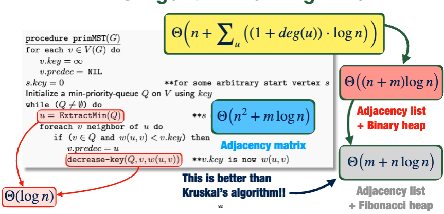
Running Time
- Extracting the minimum element and decreasing the key of an element in the priority queue is \(\Theta(\log{n})\) since the queue is implemented with a binary heap.
- So, our runtime depends on how we represent the graph
- Adjacency matrix: \(\Theta(n^2+m\log{n})\)
- Adjacency list and binary heap: \(\Theta((n+m)\log{n})\)
- Adjacency list and Fibonacci heap: \(\Theta(m+ n\log{n})\)
Aside: Cuts
- The minimum weight edge in every cutset of a graph belongs to its minimum spanning tree (up to unique edge weights)
Shortest Path (Topic 13-14)
- Shortest-path problem: given an edge-weighted graph, find the shortest path connecting a source \(s\) and a destination \(t\)
- Subpath optimality: The shortest path between any two points on the shortest path between \(s\) and \(t\) is a subpath of the shortest path between \(s\) and \(t\)
- Metric of shortest distances: for any \(u\), \(v\), \(w\) we have
- \(d(u, v) = d(v, u)\), assuming \(G\) is undirected
- \(d(u, u) = 0\)
- Triangle inequality: \(d(u, w) \leq d(u, v) + d(v, w)\) Assuming there are no negative cycles. This a reasonable assumption, since if one of these did exist, we could just go around it over and over to get an arbitrarily low cost
From MST to Shortest Path
- For MST, we keep connecting a node (via predecessor) to its smallest-cost neighbour
- For shortest path, if we find a difference between two nodes that is smaller than the previous ones, we update the distance values to match this, then set predecessors and decrease keys like for MST
Dijkstra's Algorithm
Overview
- For each adjacent node \(v\) of \(u\)
- We find the best overestimate (weight of path connecting to it)
- I.e. update \(v.dist = u.dist + w(u, v)\) for every neighbour \(v\) of \(u\)
- Then, when nodes may overlap, \(v.dist = \min{\set{u.dist + w(u, v) , v.dist}}\)
- This creates a BFS tree
- Note that we can dequeue a node once we've found that there aren't any shorter paths
- E.g. the node adjacent to the starting point of minimum weight cannot have a shorter path going through another node by definition, so it gets dequeued after the adjacencies of the first node have been considered
Pseudocode
// G is the graph, G = (V, E)
// w is the weights
// s is the starting ndoe
void dijkstra(G, w, s) {
    for(each v) {
        v.dist = infinity
        v.predec = NULL
    }
    // distance to self is 0
    s.dist = 0

    Build a Min-Priority-Queue Q on all nodes, key = dist
    // Q is the set of nodes whose shortest paths we are not sure about
    // while we still have nodes to consider:
    while(Q != []) {
        // get the closest node
        u = ExtractMin(Q)
        for(each v neighbour of u) {
            // if we find a shorter path going through an existing subpath
            // update to make that path the new shortest path
            // this is called RELAXATION
            if(v.dist > u.dist + w(u, v)) {
                v.dist = u.dist + w(u, v)
                v.predec = u
                decrease-key(Q, v, v.dist)
            }
        }
        ??? dequeue(u)
    }
}
Relaxation
- Relaxation property: For any \(v\), if \(v.dist\) is only updated using \(relax(u, v)\), then \(v.dist \leq d(s, v)\) always holds
- \(relax(u, v)\) is the following code from the algorithm:
if(v.dist > u.dist + w(u, v)) {
    v.dist = u.dist + w(u, v)
}
- This follows from the fact that none of the weights can be negative
- \(relax(u, v)\) cannot increase \(v.dist\), so whenever \(v.dist = d(s, v)\), we don't change \(v.dist\)
Correctness
Loop invariant: At the beginning of each while-loop iteration for node \(u\), we claim:
\(u.dist=d(s, u)\) for all \(u\) that aren't in the queue (i.e. \(u\in V-Q\)), i.e. nodes we aren't considering anymore
\(u.dist \geq d(s, u)\) for all \(u\) that are in the queue (i.e. \(u\in Q\))
- Initialization: clearly these are true when \(Q\) holds all the nodes
- Termination: \(Q\) will be empty, so we have found all the shortest path distances from \(s\)
- Maintenance: Suppose a node \(u\) is incorrectly dequeued, i.e. dequeued when \(d(s, u)<u.dist\)
- Let \(x\) be the last sure node before \(u\), and \(y\) is the first unsure node after \(x\) (possibly \(u\))
- We have \(y.dist \leq x.dist + w(x, y)=d(s, x)+w(x, y)=d(s, y)\), we must have already relaxed \(y\) in the last iteration
- So \(y.dist = d(s, y)\leq d(s, u)<u.dist\) by subpath optimality and non-negative edge weights
- Case 1: if \(u\) is \(y\), we have a contradiction.
- Case 2: if \(u\) is not \(y\), then the next node to be dequeued should be \(y\) instead of \(u\), still a contradiction (of \(y.dist < u.dist\))
- If we are to dequeue \(u\) from \(Q\), then the shortest path so far from \(s\) to \(u\) consists only of nodes that we are sure about; we only dequeue \(u\) once a shortest path has been found
Runtime
- Preprocessing distance and predecessors: \(O(n)\)
- Building min-priority queue: \(O(n)\)
- Extracting min and decreasing key in the min-priority queue: \(O(\log{n})\)
- Done \(n\) times, so \(O(n\log{n})\) total
- The for loop (in the while loop) is \(O(n)\) for an adjacency matrix and \(O(\deg{u})\) for the adjacency list
- So, the whole while loop is \(O(m\log{n})\) with the adjacency list
We have \(\dots < + O(n\log{n})+O(m\log{n})\), so the total runtime is \(O((n+m)\log{n})\) with an adjacency list
- Can be reduced to \(\Theta(m+n\log{n})\) with a Fibonacci heap
- With adjacency matrix, the while loop is \(n^2\), so the total runtime is \(O(n^{2}+m\log{n})\)
Drawbacks
- Does not work with non-negative edge weights
- If a weight changes, the whole algorithms needs to be re-run
Dijkstra's Algorithm for DAGs
If a graph has been sorted topologically, we already know that we don't need to "backtrack" to find a shortest path: they must move "forward" in the DAG by definition. So, we don't need to build a priority queue; we can just look at adjacent nodes in their natural order.
Pseudocode
for each vertex v {
    v.dist = infinity
    v.predec = NULL
}

s.dist = 0

for i from 1 to n-1 {
    for each u adjacent to v[i] {
        // relaxation: update the distance if needed
        if(u.dist > v[i].dist + w(v[i], u)) {
            u.dist = v[i].dist + w(v[i], u)
            u.predec = v[i]
        }
    }
}
Runtime
It takes \(O(n)\) to preprocess and \(O(m)\) to execute the for loops (since the checks happen a constant amount of time per edge). So, the total runtime is \(O(n+m)\).
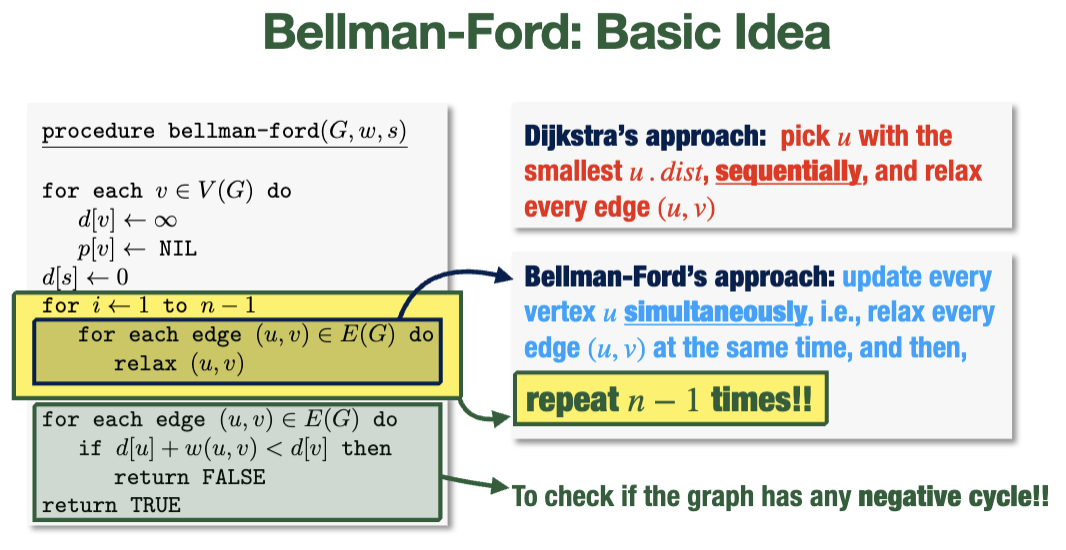
Bellman-Ford Algorithm
Slower than Dijkstra's algorithm, but can handle negative edge weights and is more flexible if the weight of an edge changes.
Idea: instead of picking the node of smallest distance sequentially, we do all of them all at once enough times that every needed relaxation can occur
Pseudocode
for each vertex v {
    v.dist = infinity
    v.predec = NULL
}

s.dist = 0

// relax each edge n times; this accounts for all the relaxations that may be needed (although it does so rather inelegantly)
for i from 1 to n-1 {
    for each edge (u, v) {
        // recall: relax checks whether a shorter path exists
        relax(u, v)
    }
}

// if things are still changing, it must be because a negative cycle exist
// (which will keep decrementing weights indefinitely)
// so, we return false in this case
for each edge (u, v) {
    if u.dist + w(u, v) < v.dist {
        return false
    }
}

return true
Runtime
The first for-loop runs in \(O(nm)\), since it executes \(n\) times and runs an \(O(1)\) procedure on each edge each time (\(O(m)\)).
Notes
The algorithm can find the shortest paths after less than \(n-1\) iterations, but still completes the rest of the computation every time.
Floyd-Warshall Algorithm
Floyd-Warshall aims to solve the All-Pairs Shortest Path problem (APSP): what is the shortest path between any two pairs of nodes in a graph?
Idea: run Dijkstra or Bellman-Ford at each vertex (\(n\) times). This would be very slow, but improvable with dynamic programming.
Subproblems
Subproblem: \(k-1\): for given vertices \(i, j\), find the distance of the shortest path from \(i\) to \(j\) where all the intermediate vertices are in \(\set{1, 2, \dots, k-1}\) (we have numbered the vertices \(1\dots n\))
- We can store this in
d[i, j, k-1]
Either we don't need vertex \(k\) (i.e. the same shortest path as subproblem \(k\) for \(i, j\)), in which case \(d[i, j, k]=d[i, j, k-1]\), or we do need \(k\), in which case \(d[i, j, k]=d[i, k, k-1]+d[k, j, k-1]\).
- We get this by following the shortest \(i\to k\) path, then the shortest \(k\to j\) path
- Sub-path optimality!
So we get the recurrence \(d[i, j, k]=\min\set{d[i, j, k-1], d[i, k, k-1]+d[k, j, k-1]}\), which is dynamic-programmable.
- Base case: \(d[i, j, 0]=w(i, j)\) or simply \(d[i, i, k]=0\).
- We can fill \(3\)-dimensional table of \(d\) bottom-up
Runtime
Our table is \(n\times n\times n\) (since it's \(3\)-dimensional and there are \(n\) nodes), so filling the entire table (which requires \(O(1)\) operations) is \(O(n^3)\).
- In comparison, running Dijkstra at each vertex is \(\Theta(n(m+n)\log{n})\) and running BF at each vertex is \(O(n^{2}m)\)
- So, these options get worse the more edges there are (i.e. in dense graphs where \(m\to n^2\)), but better in sparse graphs
Cheat Sheet
Big O \(h(n) \in O(f(n)) \iff \exists c, n_0\) such that \(\forall n \geq n_0, h(n) \leq cf(n)\)
Big Omega \(h(n) \in \Omega(f(n)) \iff \exists c, n_0\) such that \(\forall n \geq n_0, h(n) \geq cf(n)\)
Solving recurrences
- Iterated sub: We keep relacing the recursive term of the equation with its definition until it forms a pattern
- Recurrence tree: draw the recurrence tree
Let
\(a \geq 1\) and
\(b > 1\) be constants, and let
\(f(n)\) be a function. Let
\(T(n)\) be defined on non-negative integers by the recurrence
\[T(n) = aT\left(\frac{n}{b}\right)+ f(n)\] Then
\(T(n)\) has the following bounds
- If \(f(n) \in O(n^{\log_{b} {{a}- \varepsilon}})\) for some \(\varepsilon > 0\) then \(T(n) \in \Theta(n^{\log_{b}{a}})\)
- If \(f(n) \in \Theta(n^{\log_{b}{a}} \times \log^{k}{n})\) for some \(k \geq 0\) then \(T(n) \in \Theta(n^{\log_{b}{a}} \times \log^{k+1} n)\)
- If \(f(n) \in \Omega(n^{\log_{b}{a + \varepsilon}})\) for some constant \(\varepsilon > 0\) and if \(a f\left(\frac{n}{b}\right)\leq \delta f(n)\) for some constant \(\delta < 1\) and all sufficiently large \(n\), then \(T(n) \in \Theta(f(n))\)
- Finding running time
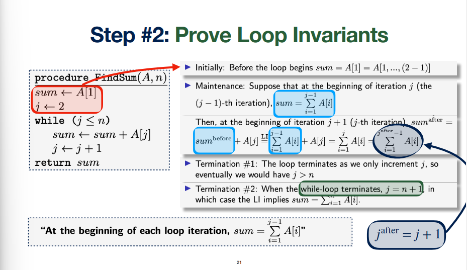
- Figure out how many times each line gets run (requires using \(\sum\limits\) for loops)
- Loop invariant: assertion that is true before loop (initialization), during the loop (maintenance), after the loop (termination 2) which has to stop (termination 1)
- Initialization like base case, maintenance is an implication \(n \implies n+1\) using what the code actually is
Heaps, Priority Queue, Heapsort
- A heap is a binary tree data structure, represented by an array, where the key of the child node is smaller than that of its parent (max heap)
- Max Heap Property: For every node \(j\), we have \(A\left[\lfloor\frac{i}{2}\rfloor\right]\geq A[j]\)
Array Indices for Heaps
Definition
- \(\text{leftchild}(A[i]) = A[2i]\)
- \(\text{rightchild}(A[i]) = A[2i+1]\)
- \(\text{parent}(A[i]) = A[\lfloor\frac{i}{2}\rfloor]\)
- Almost-heap: only root violates max-heap
- Max-heapify: almost heap into a heap \(O(\log{n})\) since run once per heap layer
- Building a heap: run max-heapify on all non-leaf nodes starting with the furthest root, move down the array until the last non-leaf node. If a switch happens, run max-heapify recursively on the parent position too (earlier in the array)
- Priority queue: implemented using a heap
- Heapsort: build array into a heap (\(n\)), first element is in order, switch A[1] and A[n], call max heapify on unsorted part since almost heap, keep doing this \(O(n \log{n})\)
Topic 6
- Quicksort overview: Divide the array into two subarrays around a pivot such that everything before the pivot is smaller than it and everything after it is larger. Then recursively quicksort each half. Finally, each half is combined, which is trivial since quicksort is sorted in place
QuickSort(A, p, r):
    // sorts A = [p ... r]
    if(p < r) {
        // A[q] is the pivot
        // all elements before q are smaller, all after are larger
        // note: partition both modifies A (side effect) AND returns q
        q = Partition(A, p, r)
        // recursive calls
        QuickSort(A, p, q-1)
        QuickSort(A, q+1, r)
    }

// Partition subprocedure
Partition(A, p, r):
    // last element of array being examined is picked as a pivot
    pivot = A[r];
    // "switch counter" (i is an index; counts up from start index)
    i = p-1
    for(j from p to r-1) { // counts up from start to second last element
        // if current element is smaller than pivot, switch and increment counter
        if(A[j] <= pivot) {
            i = i+1;
            swap(A[i], A[j])
        }
    }
    // switch last element and element in the "pivot spot", as determined by
    // incrementing i
    // note that we compared with r when switching and incrementing, so this
    // is why we can simply swap these and know the list is in the right form
    swap(A[i+1], A[r])
    return i+1
Greedy Algorithms
- We want to show that each greedy choice can replace some portion of the optimal solution, such that this altered new solution is still optimal
- Substitution property: Any optimal decision can be altered to become our greedy choices without changing its optimality (also called the greedy choice property in CLRS)
- Optimal Substructure Property: the optimal solution contains optimal solutions to subproblems that look like the original problem
- Prove with replacement argument and induction, at each point there is an optimal solution that has the same elements as the current solution
example of greedy proof here from an exam???
- Job scheduling: earliest start time first
- Activity selection: earliest finish-time first
D and C again
- power: for even \(n\), we can reduce the number of recursive calls by saving the result of \(\exp(b, \frac{n}{2})\) and squaring it. For odd \(n\), we simply call \(\exp(b, n-1)\) so that we have an even recursive call next time
- Karatsuba is like divide and conquer, but is slightly more efficient with its recursive calls
- We have \(I = w \times x\) and \(J = y \times z\)
- So, \(I \times J = w \times y \times 2^{n}+ (w\times z + x\times y) + x\times z\)
- Let \(p = w\times y\) and \(q = x\times z\), and \(r = w\times z + x\times y\)
- Notice that \((w\times z + x\times y) = r-p-q\), which requires one less multiplication to compute
- Strassen: found 7 matrices (that each take one matrix multiplication to calculate) that can be combined together with multiplication and subtraction in order to form the desired matrix product
- So, the runtime is \(O(2^{\log_2{7}})\)
DP
- Overlapping subproblems: different branches of recursive calls complete each other's work (repetition)
- Optimal substructure: the optimal solution for the overarching problem is dependant only on the optimal solutions for subproblems (dependency)
- Find a recurrence relation for the problem
- Check if the recurrence ever makes any of the same calls, and if there are reasonable amount of different ones
- What is the dependency among subproblems
- Describe array (or I guess any data structure) of values that you wish to compute. Each value will be the result of a specific recursive call
- Fill the array from the bottom up* (backward induction). Solutions to subproblems will be looked up from the array instead of being computed themselves
- Bottom up: loop over all the values up to the one we want, and fill in the array slot for each value looped over. This means we don't have to check if something is in the array because we know it will be
- Integral knapsack recurrence: \(OPT(W; w_1 \dots w_n; v_1 \dots v_n) = \max{\set{OPT(W; w_1 \dots w_{n-1}; v_1 \dots v_{n-1}), v_n + OPT(W - w_n; w_1 \dots w_{n-1}; v_1 \dots v_{n-1})}}\)
- \(LCS(x_1 \dots x_n; y_1 \dots y_m) = \max{\set{LCS(x_1 \dots x_{n-1}; y_1 \dots y_m), LCS(x_1 \dots x_{n}; y_1 \dots y_{m-1}), 1 + LCS(x_1 \dots x_{n-1}; y_1 \dots y_{m-1})}}\)
all dp examples
Graphs
BFS
// G is a graph
// s is the starting vertex

void BFS(G, s)

for each vertex v in the graph, do
    v.color = "WHITE";
    v.dist = Infinity;
    v.predec = NULL;

Initialize a queue Q

// start examining s because it is the first node
// add it to the queue and change color to grey
s.color = "GREY"
s.dist = 0
enqueue(Q, s)

while(Q !== []) {
    u = dequeue(Q)    // remove from the queue
    for each neighbour v of u {
        if(v.color = "WHITE") {
            v.color = "GREY"
            v.dist = u.dist + 1
            v.predec = u
            enqueue(Q, v)   // add v to the Queue
        }
    }
    u.color = BLACK   // done visiting the neighbours of u
}
DFS
int time  // global

void DFS(G)

    // initialize graph
    for each vertex v
        v.color = "WHITE"
        v.predec = NULL

    time = 0

    // visit all unvisited nodes
    for each vertex v
        if(v.color = "WHITE") {
            DFS-visit(G, v)
        }

void DFS-visit(G, s)

    // examining "first" node
    s.color = "GREY"
    time = time + 1
    s.dtime = time

    for each u, neighbour of s {
        if(u.color = "WHITE") {
            u.predec = s
            // recursive call
            DFS-visit(G, u)
        }
    }

    // done visiting everything
    s.color = "BLACK"
    time = time + 1
    s.ftime = time
MST
Kruskal
T = []
for each (v in V(G)) {
    Define cluster C(v) = v
}

sort edges in E(G) into non-decreasing weight order

for each (edge e = (u, v) in E(G)) {
    if(C(u) != C(v)) {
        T = [...T, e]   // union
        merge clusters C(u) and C(v)
    }
}

return T
Prim
SP
Dijkstra
// G is the graph, G = (V, E)
// w is the weights
// s is the starting ndoe
void dijkstra(G, w, s) {
    for(each v) {
        v.dist = infinity
        v.predec = NULL
    }
    // distance to self is 0
    s.dist = 0

    Build a Min-Priority-Queue Q on all nodes, key = dist
    // Q is the set of nodes whose shortest paths we are not sure about
    while(Q != []) {
        // get the closest node
        u = ExtractMin(Q)
        for(each v neighbour of u) {
            // relaxation
            if(v.dist > u.dist + w(u, v)) {
                v.dist = u.dist + w(u, v)
                v.predec = u
                decrease-key(Q, v, v.dist)
            }
        }
        ??? dequeue(u)
    }
}
or


Recursive Algorithms (Warm Up)
- How can we prove that the basic recursive factorial function is correct?
- Claim:
factorial(n) = \(n!\)
- Proof by induction
- Base case: for \(n=0\) the case holds
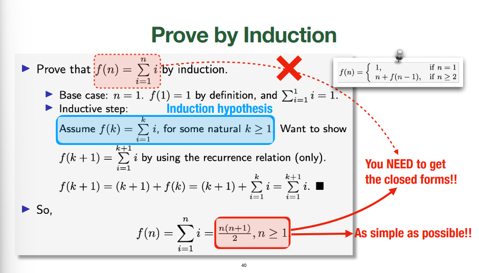
- Inductive Step (must have well-defined induction hypothesis): Let \(k \in \mathbb{N}\). Assuming the claim holds for \(k\), we show that the claim holds for \(k+1\) (i.e. \(P(k) \implies P(k+1))\)
factorial(k+1) = \((k+1)\)factorial(k) = \(\dots\) = \((k+1)!\)
- Alternative: strong induction
- If the claim holds for \(k\), \(k-1\), \(k-2\), \(\dots\) \(0\) then the claim holds for \(k+1\) as well
- Regular induction implies strong induction, it's just that strong induction needs to be used sometimes
TODO
Fast multiplication where you square values instead of recalculating them every time: was a quiz question that I ate shit on
 #### Merge Sort Application
- $T(n) =\left\{\begin{array}{lr}0 & \text{if } n=1\\2 \times T\left(\frac{n}{2}\right)+ (n-1), & \text{if } n \geq 2\end{array}\right\}$, so
- $T(2^{k})= (2^{k}- 1) + 2 \times T(2^{k}-1)$ $= (2^{k}- 1) + 2 \times ((2^{k-1} -1) + 2 \times T(2^{k-2})) = \dots$
- Eventually, by writing this out to the base case using $\dots$ and factoring, we get $k \times 2^{k}- \sum\limits^{k-1}_{i=0} 2^{i}= k\times 2^{k}- (2^{k}-1) = (k-1)2^{k}+ 1$
- Since $n=2^k$, we have $k = \log(n) \implies T(n) = n \log(n - 1) + 1$
- We have found $T(n)$, but not proven it. For that, we need induction. The induction proof follows structurally from the recurrence relation
#### Merge Sort Application
- $T(n) =\left\{\begin{array}{lr}0 & \text{if } n=1\\2 \times T\left(\frac{n}{2}\right)+ (n-1), & \text{if } n \geq 2\end{array}\right\}$, so
- $T(2^{k})= (2^{k}- 1) + 2 \times T(2^{k}-1)$ $= (2^{k}- 1) + 2 \times ((2^{k-1} -1) + 2 \times T(2^{k-2})) = \dots$
- Eventually, by writing this out to the base case using $\dots$ and factoring, we get $k \times 2^{k}- \sum\limits^{k-1}_{i=0} 2^{i}= k\times 2^{k}- (2^{k}-1) = (k-1)2^{k}+ 1$
- Since $n=2^k$, we have $k = \log(n) \implies T(n) = n \log(n - 1) + 1$
- We have found $T(n)$, but not proven it. For that, we need induction. The induction proof follows structurally from the recurrence relation